Using pose estimation to identify regions and points on natural history specimens

Abstract

A key challenge in mobilising growing numbers of digitised biological specimens for scientific research is finding high-throughput methods to extract phenotypic measurements on these datasets. In this paper, we test a pose estimation approach based on Deep Learning capable of accurately placing point labels to identify key locations on specimen images. We then apply the approach to two distinct challenges that each requires identification of key features in a 2D image: (i) identifying body region-specific plumage colouration on avian specimens and (ii) measuring morphometric shape variation in Littorina snail shells. For the avian dataset, 95% of images are correctly labelled and colour measurements derived from these predicted points are highly correlated with human-based measurements. For the Littorina dataset, more than 95% of landmarks were accurately placed relative to expert-labelled landmarks and predicted landmarks reliably captured shape variation between two distinct shell ecotypes ('crab' vs 'wave'). Overall, our study shows that pose estimation based on Deep Learning can generate high-quality and high-throughput point-based measurements for digitised image-based biodiversity datasets and could mark a step change in the mobilisation of such data. We also provide general guidelines for using pose estimation methods on large-scale biological datasets.

Fig 1. Examples of points on the avian specimen images.

(a) Five reflectance standards and five body regions (crown, nape, mantle, rump and tail) of the back view; (b) Three body regions (throat, breast and belly) of the belly view; (c) Two body regions (wing coverts and flight feathers) of the side view.

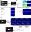
Fig 2. The pipeline of applying the Stacked Hourglass model to predict points on the avian specimen dataset.

(a) A data pre-processing step resizes images (from 4948 x 3280 pixels to 494 x 328 pixels) and transforms point coordinates into heatmaps (62 x 41 pixels). (b) This pre-processed training data is then used to train the network. Output heatmaps iteratively become closer to ground truth during training. (c) The trained network is used to generate predictions of point locations for validation images. These are then post-processed (transforming heatmaps back to coordinates) and evaluated.

Fig 3. An example of a Littorina shell image and seven landmarks.

LM1 is defined as the apex of the shell; LM2 is defined as the upper suture of the penultimate whorl (right); LM3 is defined as the upper suture of the penultimate whorl (left); LM5 is defined as the end of the suture; LM6 is defined as the point at the external edge of the lip and the line between LM4 and LM6 (white dotted line) is tangent to the operculum; LM7 is defined as the point at the bottom of the shell and the line between LM1 and LM7 (red dotted line) is tangent to the aperture.

Fig 4. Evaluation results between ground truth and predictions for the avian specimen dataset.

(a) Pixel distances. The x axis (pixel distance) is logarithmic scaled; (b) PCK-100; (c) RGB Colour correlations (colour extraction method: Heatmap-90).

Fig 5. Example images of ground truth and predictions for the avian specimen dataset.

Images (a)-(d) are correct predictions: (a) a specimen with high colour diversity, (b) a big specimen and very small reflectance standards, (c) a specimen with interferential objects such as a specimen tag, (d) a specimen which is similar to the background. Images (e)-(h) are incorrect predictions: (e) The tail is partially occluded by a wing, and it was incorrectly labelled as the wing. (f) The eye of the bird was misidentified as the crown, while the specimen was placed in a rare posture (placed on its back rather than belly) in the image. (g) The predictions of the wing were placed on the body, and the wing has a similar colour to the rest of the body regions. (h) The predictions were not placed on the wing which is very small. (Note: we cropped only focal parts of images to achieve better visualisation).

Fig 6. Pixel distances for experts and Deep Learning comparison.

Pixel distances are compared across three groups: predictions vs expert trainer (PvT); predictions vs expert non-trainer (PvNT); between experts (EvE). Red dotted lines are the median of PvT. Significant symbols are t-test that compares PvT against PvNT or EvE (ns: p > 0.05; *: p < = 0.05; **: p < = 0.01; ***: p < = 0.001; ****: p < = 0.0001). All Y axes (pixel distance) are square root scaled.

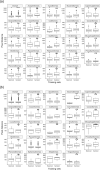
Fig 7. Pixel distances for balance and imbalance in taxonomic groups comparison.

(a) Comparing the performance between using the balanced training set and using the imbalanced training set on the balanced test set. (b) Comparing the performance between using the balanced training set and using the imbalanced training set on the imbalanced test set. The performance was evaluated on the pixel distance. Significant symbols are t-test results (ns: p > 0.05; *: p < = 0.05; **: p < = 0.01; ***: p < = 0.001; ****: p < = 0.0001). All Y axes (pixel distance) are square root scaled.

Fig 8. Distributions of PC1 and 2 for Littorina shells.

PC1 and PC2 explains 62.9% of the total variation. Left: the ground truth landmarks (Crab: Grey; Wave: Yellow). Right: Deep Learning predicted landmarks (Crab: Blue; Wave: Red).

References

1. Jarvis ED, Mirarab S, Aberer AJ, Li B, Houde P, Li C, et al.. Whole-genome analyses resolve early branches in the tree of life of modern birds. Science. 2014. Dec 12;346(6215):1320–31. doi: 10.1126/science.1253451 - DOI - PMC - PubMed
1. Zhang G, Li C, Li Q, Li B, Larkin DM, Lee C, et al.. Comparative genomics reveals insights into avian genome evolution and adaptation. Science. 2014. Dec 12;346(6215):1311–20. doi: 10.1126/science.1251385 - DOI - PMC - PubMed
1. Lussier YA, Liu Y. Computational Approaches to Phenotyping: High-Throughput Phenomics. Proceedings of the American Thoracic Society. 2007;4(1):18–25. doi: 10.1513/pats.200607-142JG - DOI - PMC - PubMed
1. Lürig MD, Donoughe S, Svensson EI, Porto A, Tsuboi M. Computer Vision, Machine Learning, and the Promise of Phenomics in Ecology and Evolutionary Biology. Frontiers in Ecology and Evolution. 2021;9(April).
1. Ariño A. Approaches to estimating the universe of natural history collections data. Biodiversity Informatics. 2010;7(2):81–92.
Publication types