Embracing enzyme promiscuity with activity-based compressed biosensing

Abstract

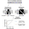
The development of protease-activatable drugs and diagnostics requires identifying substrates specific to individual proteases. However, this process becomes increasingly difficult as the number of target proteases increases because most substrates are promiscuously cleaved by multiple proteases. We introduce a method-substrate libraries for compressed sensing of enzymes (SLICE)-for selecting libraries of promiscuous substrates that classify protease mixtures (1) without deconvolution of compressed signals and (2) without highly specific substrates. SLICE ranks substrate libraries using a compression score (C), which quantifies substrate orthogonality and protease coverage. This metric is predictive of classification accuracy across 140 in silico (Pearson r = 0.71) and 55 in vitro libraries (r = 0.55). Using SLICE, we select a two-substrate library to classify 28 samples containing 11 enzymes in plasma (area under the receiver operating characteristic curve [AUROC] = 0.93). We envision that SLICE will enable the selection of libraries that capture information from hundreds of enzymes using fewer substrates for applications like activity-based sensors for imaging and diagnostics.

Keywords: activity-based sensor; compressed sensing; protease; protease-activatable drugs; substrate selection; synthetic biomarker.

Graphical abstract

Figure 1

Conceptual overview of protease substrate design using the SLICE method (1) Identify which proteases in the system being probed are considered target proteases (blue Pacman) and which are off-target proteases (purple Pacman). (2) Generate candidate peptide sequences that can be used as substrates for target proteases. Peptide sequences can be acquired from the literature (paper icon) or computationally generated (computer icon). Computationally generated diversity includes degenerate libraries as well as predicted sequences derived from computational modeling software. (3) Screen candidate peptide sequences against all protease targets via chemically synthesized activity-based sensors (e.g., fluorogenic probes, peptide microarrays, etc.) or genetically encoded libraries (e.g., phage display, bacteria display, etc.). (4) Heatmap of cleavage kinetics, quantified by the catalytic constant, k_cat, for all protease-substrate pairs (rows = proteases, columns = substrates). (5a) An example promiscuous substrate library that has fewer substrates (n_substrates = 5) than proteases (n_proteases = 10). The compression score, C, represents the score assigned to the library by the SLICE method, with 1 being the highest score and 0 the lowest. (5b) An example specific substrate library that has the same number of substrates as proteases (n_substrates = n_proteases = 10).

Figure 2

Computational pipeline for evaluating classification performance of simulated substrate libraries (1a) Plot of first two principal components from principal-component analysis on microarray gene expression data of 162 protease genes in day 1 (healthy, blue) and 7 (disease, red) mouse tissue samples in a B16 melanoma model. To simulate, 100 samples and 100 disease samples are computationally generated as a Gaussian distribution from a single biological sample. (1b) Heatmap of simulated catalytic constatnts, k_cat, for every pairwise combination between 162 proteases and 150 substrates (white = high, black = low). (2) Visualization of how product formation rates, V_max, are calculated using protease concentrations, P, and k_cat. The result of this calculation is a product formation rate per substrate per sample. (3) Receiver operating characteristic (ROC) curves as a measure of healthy versus disease classification performance using product formation rates as features of observations used to train a random forest model. Blue trace is an ROC curve when using signals (i.e., product formation rates) from 11 substrates (green trace = 5 substrates, red trace = 1 substrate).

Figure 3

A compression score for promiscuous substrate selection (A) Equation used to calculate the compression score, C. Substrate orthogonality, S_orth., which is quantified by the cosine distance metric, and protease coverage, P_cov., which quantifies the fraction of proteases that are sampled by a substrate library, are combined according to the weight of summation, ω. All variables range from 0 to 1. (B) Schematic showing four example substrate libraries and their relative magnitude in S_orth. (y axis) and P_cov. (x axis) space. Each substrate library is represented with a heatmap of catalytic constats, k_cat, (white = high, black = low) for all protease (rows) and substrate (columns) combinations. (C) (Top) Schematic showing pipeline for calculating C and classification performance for 140 simulated substrate libraries. (Bottom) Plot of correlation between C (x axis) and classification performance (AUROC, y axis). Black line is line of best fit. Each dot represents the performance of one substrate library averaged over 5 repeats. (D and E) Plots showing classification performance (AUROC, y axis) versus substrate library size (number of substrates, x axis) for changing value of S_orth. (D) and P_cov. (E). Each dot represents the performance of one substrate library.

Figure 4

Exhaustive scoring of substrate libraries in vitro with SLICE (A) (1, left) Schematic of activity sensor or fluorogenic probe. Activity sensor comprises a peptide substrate (blue and red bar) flanked with a fluorophore (yellow star = 5-FAM, red star = EDANS) and a quencher (black circle = Dabcyl). Upon cleavage, the fluorophore and quencher separate, which results in an increase in fluorescent signal. (1, right) Cleavage assay of thrombin and substrate-1 showing the increase in number of substrates cleaved (y axis) over time (x axis). Black dots are raw data. The slope (triangle) of the line of best fit (black line) is calculated as the product formation rate. Relative fluorescence unit (RFU)/min is used as RFU correlates with the number of substrates cleaved. (2) Heatmap showing all pairwise combinations of product formation rates as measured from independent cleavage assays. Proteases are in rows, and substrates are in columns. Data are natural log transformed. (B) (1) Schematic showing that all unique combinations of substrates, with library sizes ranging from 2 to 10, are scored with SLICE. (2) Histogram showing the distribution of S_orth. (red distribution) and P_cov. (blue distribution) scores. (3) Histogram showing the distribution of the compression score, C (light blue distribution). Vertical dashed lines depict the score of various controls. “No sensing” depicts the score of a library where kinetic constant = 0 for all protease-substrate pairs. “Randomly generated” depicts the score of a library where kinetic constants are randomly generated. “Perfect orthog. & coverage’ depicts the score of a library where all proteases are sampled, and each substrate has no overlapping kinetic constants. (C) (1) Principal-component analysis of 11 proteases selected from 162 found in original B16 study. Proteases selected as either exact match or as member of same family as 11 proteases used in our study (A, part 2). Each dot represents one simulated sample (red = disease, blue = healthy). (2) Histogram showing the distribution of Cs (light blue distribution) for all substrate libraries of size 2 (i.e., 2 substrates). (3) Plot showing correlation between C (x axis) and classification performance (y axis, AUROC). Black line shows line of best fit.

Figure 5

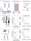
Experimental validation of substrate library design with SLICE (A) Schematic of experimental workflow: (1) Two mixtures (A = blue, B = red) of 11 proteases are randomly generated. Each mixture is represented with a test tube containing 11 proteases (Pacman shape). Relative size of protease roughly represents the relative concentration. Actual relative concentrations are plotted in bar graph below (A = blue bars, B = red bars). (2) Schematic of experimental well plate containing samples of protease mixtures (1 circle = 1 well). Both mixtures are independently pipetted 10 times each (blue well = mix A, red well = mix B) to create a population with variance due to pipetting error. One library is introduced to all 20 samples (10 of mixture A, 10 of mixture B), and the product formation rates of both activity-based sensors in the library are measured. (3) Schematic graph (not real data) showing that the library with a high compression score, C, (C > 0.9) should have high classification performance (blue line), whereas the library with low C (C < 0.5) should have low classification performance (orange line). (B) Heatmaps showing the product formation rates for the library with the highest C (C = 0.95 library) and the library with the lowest C (C = 0.49 library) (white = high product formation rate, black = low product formation rate). (C) Plot of the resulting product formation rates for each activity sensor after incubation with protease mixtures (1 dot = 1 mixture; blue dot = mixture A, red dot = mixture B). The product formation rates from activity-based sensors using 5-FAM are plotted on the x axis, and product formation rates from EDANS are plotted on the y axis. The top plot shows the results when using the C = 0.49 library, and the bottom plot shows the results when using the C = 0.95 library. Rates were normalized from 0 to 1 for visualization. (D) AUROC plot showing the results of classifying mixture A from mixture B when using the C = 0.95 library (blue trace) or the C = 0.49 library (orange trace). (E) Schematic of workflow to test classification in citrated plasma. (F) Plot of product formation rates for each activity sensor after incubation with protease mixture A or B in the presence of citrated plasma (plasma was isolated from 5 mice, and assay was performed with 2–3 technical replicates each, for total of n = 14). (G) AUROC plot showing classification results in plasma.

References

1. Bond J.S. Proteases: history, discovery, and roles in health and disease. J. Biol. Chem. 2019;294:1643–1651. - PMC - PubMed
1. Barrett A.J., Rawlings N.D., Woessner J.F. In: Handbook of Proteolytic Enzymes. Second Edition. Barrett A.J., Rawlings N.D., Woessner J.F., editors. Academic Press; 2004. Introduction. pp. xxxiii–xxxv.
1. López-Otín C., Bond J.S. Proteases: multifunctional enzymes in life and disease. J. Biol. Chem. 2008;283:30433–30437. - PMC - PubMed
1. Sanman L.E., Bogyo M. Activity-based profiling of proteases. Annu. Rev. Biochem. 2014;83:249–273. - PubMed
1. Turk B. Targeting proteases: successes, failures and future prospects. Nat. Rev. Drug Discov. 2006;5:785–799. - PubMed
Publication types
MeSH terms
LinkOut - more resources