. 2023 Jan 31;13(2):245.
doi: 10.3390/brainsci13020245.

Biologically-Based Computation: How Neural Details and Dynamics Are Suited for Implementing a Variety of Algorithms

Affiliations

Biologically-Based Computation: How Neural Details and Dynamics Are Suited for Implementing a Variety of Algorithms

Nicole Sandra-Yaffa Dumont et al. Brain Sci. .

Abstract

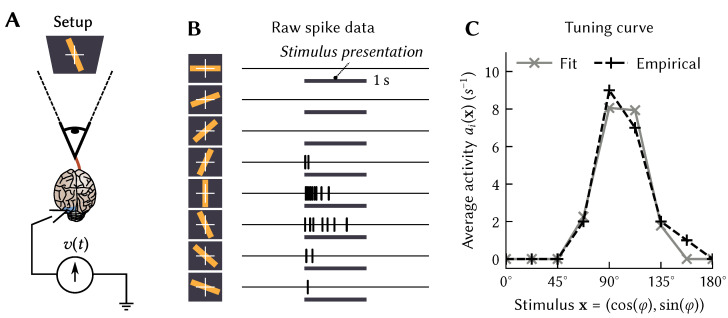
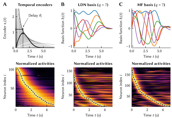
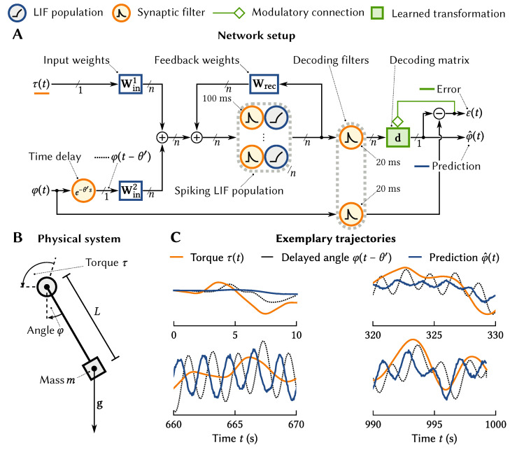
The Neural Engineering Framework (Eliasmith & Anderson, 2003) is a long-standing method for implementing high-level algorithms constrained by low-level neurobiological details. In recent years, this method has been expanded to incorporate more biological details and applied to new tasks. This paper brings together these ongoing research strands, presenting them in a common framework. We expand on the NEF's core principles of (a) specifying the desired tuning curves of neurons in different parts of the model, (b) defining the computational relationships between the values represented by the neurons in different parts of the model, and (c) finding the synaptic connection weights that will cause those computations and tuning curves. In particular, we show how to extend this to include complex spatiotemporal tuning curves, and then apply this approach to produce functional computational models of grid cells, time cells, path integration, sparse representations, probabilistic representations, and symbolic representations in the brain.

Keywords: cognitive modelling; neural engineering framework; spatial semantic pointers; spatiotemporal representation; time cells.


Conflict of interest statement

T.C.S. and C.E. have a financial interest in Applied Brain Research, Incorporated, holder of the patents related to the material in this paper (patent 17/895,910 is additionally co-held with the National Research Council Canada). The company or this cooperation did not affect the authenticity and objectivity of the experimental results of this work. The funders had no role in the direction of this research; in the analyses or interpretation of data; in the writing of the manuscript; or in the decision to publish the results.

Figures

Figure 1
Figure 1
Illustration of the original Hubel and Wiesel experiment [15]. (A) Measuring the activity ai of a neuron in response to a bar of light projected onto a screen. (B) The neuron produces different levels of activity depending on the orientation of the bar of light x (data from [15]). (C) Plotting the activity ai(x) (dashed line) and a least-squares fit G[J(x)] (gray line; G is a LIF response curve).
Figure 2
Figure 2
Examples of tuning curves in the linear-nonlinear tuning-curve family with a LIF nonlinearity G. (A) Using d=1 results in monotonic tuning over a quantity x. Coloured lines correspond to individual neurons i. (B) Bell-shaped tuning-curves can be obtained with d=2 and transforming x=(sin(πx),cos(πx)). (C) Tuning curve of a single hexagonal grid cell constructed using spatial semantic pointers (SSPs) with d=7 (deep blue corresponds to a firing rate of 100 Hz).
Figure 3
Figure 3
Model of a neuron in visual cortex tuned to downwards motion. The spatiotemporal encoder e is a two-dimensional Gabor filter sampled in two spatial dimensions ξ1, ξ2 that correspond to coordinates in the visual field [25,26]. (A,B) Different slices through e. Blue corresponds to positive, red to negative values. (C) Computing the neural activity for a grating pattern x moving in the arrow direction. Downwards motion results in the strongest response amplitude.
Figure 4
Figure 4
Transforming signals. (A) Two LIF neuron populations (blue, green) are tuned to variables x, y. The first population projects onto to the second; we impose the relationship y=f(x)=x2 when solving for weights. The black “neuron” is a linear readout with G[J]=J. (B) Tuning curves of the neurons depicted in (A). Left column depicts the tuning curves over x, right column the tuning curves over y. The tuning of the first (blue) population is undefined with respect to y. When controlling the stimulus variable x the network implicitly computes f(x)=x2. (C) Spike raster of the two LIF populations when varying the stimulus x over time; although we solve for weights using a rate approximation G[J], the resulting network is compatible with spiking neurons.
Figure 5
Figure 5
Realising time cells in NEF networks. (A) Top: Manually selected temporal encoders ei modelling core properties of biological time cells: bias towards shorter delays θi, and larger spread in activity for larger θi. Bottom: Activities of 200 recurrently connected integrate-and-fire neurons in response to a positive pulse after solving for weights realising the ei. Activities are normalised to the maximum activity of each neuron (yellow). Only active neurons are depicted; 50% of the neurons are “off”-neurons that react to negative input pulses. (B,C) Qualitatively similar activities can be obtained when selecting a linear combination of temporal basis functions as temporal encoders. The basis functions depicted here are the impulse response of the Legendre Delay Network (LDN) and the Modified Fourier (MF) Linear Time Invariant (LTI) systems for q=7. Having closed-form state-space LTI systems with matrices (A,B) simplifies solving for recurrent weights in the NEF.
Figure 6
Figure 6
Using neurons with time cell tuning to predict nonlinear pendulum dynamics. (A,B) Overview of the experimental setup. The torque τ(t) and a delayed angle φ(tθ) are fed into a recurrent neural network with time-cell tuning over two dimensions. We use the delta learning rule to learn connection weights online that recombine the neural activities to predict the angle in θ seconds. (C) The system learns to predict the pendulum angle with a normalized RMSE of about 20%.
Figure 7
Figure 7
One trial of LLP learning to predict the motion of a ball bouncing off the walls of a box with lossless collisions. (A) Initially the system cannot predict the future motion of the ball. (B) Using a LDN dimensionality of q=10, the LLP learns to predict the future motion of the ball. (C) shows the windowed mean (window of 1 s) of the root mean square error of the predicted path for the LLP algorithm with three different context representations over 100 trials. The LDN context uses an LDN to summarize the recent motion of the ball. The SSP context encodes the current position of the ball, and the SSP Speed context encodes the position and velocity of the ball. For each context encoding we used the largest learning rate that provided a stable learning rule. The solid line is the average performance, and the shaded regions (not visible in plot) represent a 95% confidence interval. While the SSP algorithms learn more slowly than the LLP with the LDN context, they ultimately reach lower prediction error. In all cases, by working in the LDN’s compressed representation we can learn to predict delayed signals, updating historical predictions with simple linear operations.
Figure 8
Figure 8
(A) Illustration of the projection to the frequency domain of the SSP space given in Equation (4). The dot products between a 2D variable x and a set of three vectors {aj} are cast as the phases of a set of phasors, {eiaj·x}, which reside on the unit circle in the complex plane. The IDFT of the vector [eia0·x,eia1·x,eia3·x] is a SSP representation of x, which resides in a higher dimensional vector space. In this example, the SSP is only 3-dimensional, but in practice a much larger set {aj} is used to produce high dimensional SSPs. (B) Consider how these phasors change for a x traversing 2D space. The banded heat maps shows how the real part of the vectors {eiaj·x} repeats over a 2D region of x values. Each component of the SSP in the Fourier domain is a plane wave with wave vector aj. The gridded heat map is the similarity between the SSP representation of x from (A) and SSPs of neighboring points: ϕ(x)·ϕ(x). The similarity map is periodic due to the inference pattern of all plane waves. Here a hexgaonlly gridded similarity pattern is obtained.
Figure 9
Figure 9
Map encoding using SSPs. (A) A 2D environment consisting of a rat, walls, and cheese. Information about the objects and their locations was encoded in single vector E, as per Equation (5). (B) The vector E was queried for the location of the rat by approximate unbinding: ER1ϕ(x1,y1)+ noise. The cosine similarity between the query output and SSP representations of points gridded over 2D space was computed and plotted to produce the above heat map. (C) The similarity map obtained from querying the map E for the location of cheese. (D) The similarity map obtained from querying for the wall area.
Figure 10
Figure 10
Firing patterns of LIF neurons representing SSPs. (A) A grid cell from a population encoding ϕ(x(t)), where x(t) is the path shown in grey (obtained from [58]). Red dots indicate the positions at which the cell fired. (B) A place cell from a population encoding ϕ(x(t)). (C) An object vector cell from a population encoding the SSP representation of the vector between x(t) and any objects in view. Object locations are marked with an ‘x’. (D) A border cell from a population encoding the SSP representation of the vector between x(t) and a wall along the right side of the environment.
Figure 11
Figure 11
Mean reward gained over 200 learning trials for each configuration of the Actor-Critic network exploring how sparsity (proportion of neurons active at any given time) and number of neurons impacts network performance on a spatial reinforcement learning task (MiniGrid).
Figure 12
Figure 12
The path integration model results on a 60 s long 2D path (a rat’s trajectory running in a cylinder with a diameter of 180 cm; obtained from [51]). The grey line is the ground truth. As input the model received a initial position and the velocity along the path (computed via finite differences). The output of the model was a position estimate, in the form of an SSP, over time. The 2D path estimate plotted as a black dashed line was decoded from the raw SSP output.
Figure 13
Figure 13
Results from temporal integration of SSPs to obtain trajectory representations. Path integration was performed on a 2D path (the black line in (B)). The output of the path integrator was fed into a temporal integrator, with dynamics given by Equation (10). (A) Two panels show the x-dimension of the trajectory output at different points (indicated by black stars) over the simulation time (the x axis). The output Φ(t) is visualized by a contour plot of its similarity with SSP representations across x-space. This is analogous to a probability distribution of the x position at different points in the past (see Section 6). (B) The 2D trajectory estimate, decoded from Φ(t) at the end of the simulation, as a blue line that fades with how far the estimate is into the past.
Figure 14
Figure 14
Kernel Density Estimators (KDEs; green line) approximate probability distributions (shaded region). Using the Spatial Semantic Pointer representation we can approximate the Fourier Integral Estimator (FIE)—a density estimator using a sinc kernel function. More importantly, we can represent probability with finite neural resources, and interpret operations on that representation as probability statements. Figure adapted from [66].
Figure 15
Figure 15
The regret performance of Bayesian optimization implemented using Gaussian processes with a Matern kernel (GP-BO Matern) and implemented using the Hexagonal Spatial Semantic Pointer representation (SSP-BO Hex) on the Himmelblau standard optimization test function (A). The regret performance of SSP-based algorithms is statistically equivalent to the GP methods, however, by working in the neurally-plausible feature spaces, the computation time becomes constant in the number of samples collected (B). Figured adapted from [65].

Similar articles

Cited by

References

    1. Eliasmith C., Anderson C.H. Neural Engineering: Computation, Representation, and Dynamics in Neurobiological Systems. MIT Press; Cambridge, MA, USA: 2003.
    1. Eliasmith C., Stewart T.C., Choo X., Bekolay T., DeWolf T., Tang Y., Rasmussen D. A Large-Scale Model of the Functioning Brain. Science. 2012;338:1202–1205. doi: 10.1126/science.1225266. - DOI - PubMed
    1. Choo X. Ph.D. Thesis. University of Waterloo; Waterloo, ON, Canada: 2018. Spaun 2.0: Extending the World’s Largest Functional Brain Model.
    1. Reed S., Zolna K., Parisotto E., Colmenarejo S.G., Novikov A., Barth-Maron G., Gimenez M., Sulsky Y., Kay J., Springenberg J.T., et al. A generalist agent. arXiv. 20222205.06175
    1. Silver D., Huang A., Maddison C.J., Guez A., Sifre L., Van Den Driessche G., Schrittwieser J., Antonoglou I., Panneershelvam V., Lanctot M., et al. Mastering the game of Go with deep neural networks and tree search. Nature. 2016;529:484–489. doi: 10.1038/nature16961. - DOI - PubMed

LinkOut - more resources