Using a latent Hawkes process for epidemiological modelling

Abstract

Understanding the spread of COVID-19 has been the subject of numerous studies, highlighting the significance of reliable epidemic models. Here, we introduce a novel epidemic model using a latent Hawkes process with temporal covariates for modelling the infections. Unlike other models, we model the reported cases via a probability distribution driven by the underlying Hawkes process. Modelling the infections via a Hawkes process allows us to estimate by whom an infected individual was infected. We propose a Kernel Density Particle Filter (KDPF) for inference of both latent cases and reproduction number and for predicting the new cases in the near future. The computational effort is proportional to the number of infections making it possible to use particle filter type algorithms, such as the KDPF. We demonstrate the performance of the proposed algorithm on synthetic data sets and COVID-19 reported cases in various local authorities in the UK, and benchmark our model to alternative approaches.

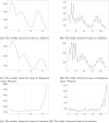
Fig 1. The generation interval (GI) (black curve) and the period between observed and actual infection times (red curve).

Fig 2. Weekly Observed Data (Scenario A (black line); Scenario B (red line)) plotted against time.

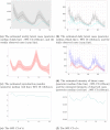
Fig 3. The true (black line) and the estimated weighs {Rn}n=116, weekly latent cases and latent intensity (with estimated seeds (posterior median (brown line); 99% CI (cyan line)), and true seeds (posterior median (red line; 99% CI (green line))) in Scenario A plotted against time.

The vertical dotted lines show the beginning of each week in the period we examine. (a) ${\left\{R_n\right\}}_{n=1}^{16}$. (b) Weekly latent cases. (c) Intensity of latent cases.

Fig 4. The true (black line) and the estimated weighs {Rn}n=116, weekly latent cases and latent intensity (with estimated seeds (posterior median (brown line); 99% CI (cyan line)), and true seeds (posterior median (red line); 99% CI (green line))) in Scenario B plotted against time.

The vertical dotted lines show the beginning of each week in the period we examine. (a) ${\left\{R_n\right\}}_{n=1}^{16}$. (b) Weekly latent cases. (c) Intensity of latent cases.

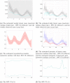
Fig 5. The weekly observed cases, the estimated intensity, the estimated reproduction number, the estimated weekly hidden cases using KDPF(median (red line); 99% CI (cyan line)), using APF (median (brown line); 99% CI (green dashed lines)), using PMMH (median (aquamarine line); 99% CI (grey dashed lines)), using BF (median (blue line); 99% CI (pink dashed lines)) and the true values (black line) in scenario C plotted against time.

The vertical dotted lines show the beginning of each week in the period we examine. (a) The weekly observed cases. (b) The estimated intensity of latent cases. (c) The estimated weights ${\left\{R_n\right\}}_{n=1}^{16}$. (d) The estimated weekly hidden cases.

Fig 6. The daily and weekly observed infections in local authorities plotted against time.

(a) The weekly observed cases in Ashford. (b) The daily observed cases in Ashford. (c) The weekly observed cases in Kingston upon Thames. (d) The daily observed cases in Kingston upon Thames. (e) The weekly observed cases in Leicester. (f) The daily observed cases in Leicester.

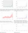
Fig 7. The weekly and daily latent cases, the reproduction number, the latent and observed intensity and the 99% CIs of time-constant parameters in Ashford plotted against time.

The time interval between two successive pink vertical dashed lines corresponds to a week. (a) The estimated weekly latent cases (posterior median (black line); 99% CI (ribbon)), and the weekly observed cases (cyan line). (b) The estimated daily latent cases (posterior median (black line); 99% CI (ribbon)), and the daily observed cases (cyan line). (c) The estimated reproduction number (posterior median (red line); 95% CI (ribbon)). (d) The estimated intensity of latent cases (posterior median (blue line); 99% CI (ribbon)) and the estimated intensity of observed cases (posterior median (red line); 99% CI (ribbon)). (e) The 99% CI of d. (f) The 99% CI of v.

Fig 8. The weekly and daily latent cases, the reproduction number, the latent and observed intensity and the 99% CIs of time-constant parameters in Kingston upon Thames plotted against time.

The time interval between two successive pink vertical dashed lines corresponds to a week. (a) The estimated weekly latent cases (posterior median (black line); 99% CI (ribbon)), and the weekly observed cases (cyan line). (b) The estimated daily latent cases (posterior median (black line); 99% CI (ribbon)), and the daily observed cases (cyan line). (c) The estimated reproduction number (posterior median (red line); 95% CI (ribbon)). (d) The estimated intensity of latent cases (posterior median (blue line); 99% CI (ribbon)) and the estimated intensity of observed cases (posterior median (red line); 99% CI (ribbon)). (e) The 99% CI of d. (f) The 99% CI of v.

Fig 9. The weekly and daily latent cases, the reproduction number, the latent and observed intensity and the 99% CIs of time-constant parameters in Leicester plotted against time.

The time interval between two successive pink vertical dashed lines corresponds to a week. (a) The estimated weekly latent cases (posterior median (black line); 99% CI (ribbon)), and the weekly observed cases (cyan line). (b) The estimated daily latent cases (posterior median (black line); 99% CI (ribbon)), and the daily observed cases (cyan line). (c) The estimated reproduction number (posterior median (red line); 95% CI (ribbon)). (d) The estimated intensity of latent cases (posterior median (blue line); 99% CI (ribbon)) and the estimated intensity of observed cases (posterior median (red line); 99% CI (ribbon)). (e) The 99% CI of d. (f) The 99% CI of v.

Fig 10. The estimated weekly observed cases (posterior median (red line); 95% CI (ribbon)) and the actual cases (black line) plotted against time.

(a) Ashford. (b) Kingston upon Thames. (c) Leicester.

Fig 11. The weekly average of daily estimates of the reproduction number via posterior median derived by the method of Koyama et al. [10] (blue line) and the posterior medians of R(t) given by EpiEstim (brown line) and the proposed algorithm (red line) plotted against time.

(a) Ashford. (b) Kingston upon Thames. (c) Leicester.

Fig 12. The estimated daily number of events derived by the method of Koyama et al. [10] (brown line), the estimated latent intensity (posterior median (blue line); 99% CI (ribbon)) and the estimated intensity of observed cases (posterior median (red line); 99% CI (ribbon)) plotted against time.

(a) Ashford. (b) Kingston upon Thames. (c) Leicester.

References

1. Ferguson, N., Laydon, D., Nedjati Gilani, G., Imai, N., Ainslie, K., Baguelin, M., et al. Report 9: Impact of non-pharmaceutical interventions (NPIs) to reduce COVID-19 mortality and healthcare demand. (Imperial College in London, 2020). 10.25561/77482 - DOI
1. Chen, Y., Cheng, J., Jiang, Y. & Liu, K. A time delay dynamic system with external source for the local outbreak of 2019-nCoV. Applicable Analysis. pp. 1-12 (2020)
1. Wangping J., Ke H., Yang S., Wenzhe C., Shengshu W., Shanshan Y., et al.. Extended SIR prediction of the epidemics trend of COVID-19 in Italy and compared with Hunan, China. Frontiers In Medicine. 7 pp. 169 (2020) doi: 10.3389/fmed.2020.00169 - DOI - PMC - PubMed
1. Roques L., Klein E., Papaix J., Sar A. & Soubeyrand S. Using early data to estimate the actual infection fatality ratio from COVID-19 in France. Biology. 9, 97 (2020) doi: 10.3390/biology9050097 - DOI - PMC - PubMed
1. Zou, D., Wang, L., Xu, P., Chen, J., Zhang, W. & Gu, Q. Epidemic Model Guided Machine Learning for COVID-19 Forecasts in the United States. MedRxiv. (2020), https://www.medrxiv.org/content/early/2020/05/25/2020.05.24.20111989