Coastal phytoplankton blooms expand and intensify in the 21st century

Abstract

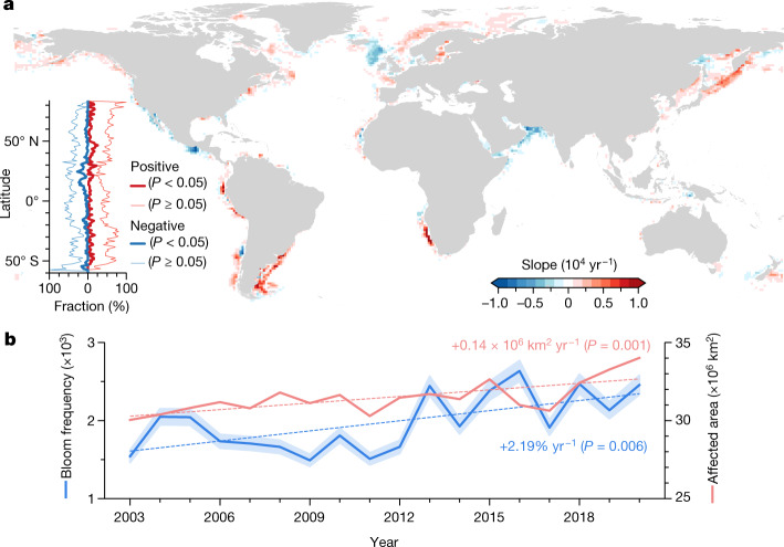
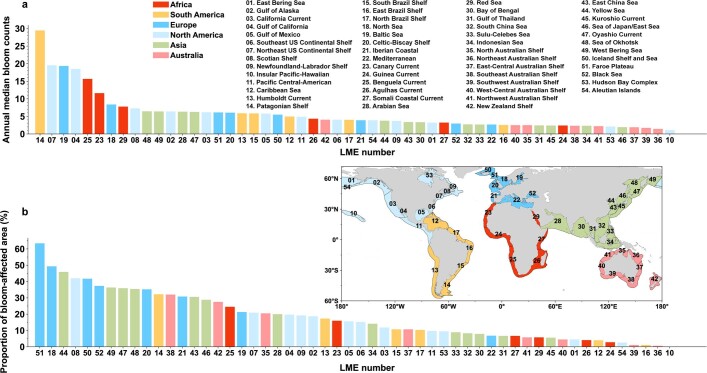
Phytoplankton blooms in coastal oceans can be beneficial to coastal fisheries production and ecosystem function, but can also cause major environmental problems^1,2-yet detailed characterizations of bloom incidence and distribution are not available worldwide. Here we map daily marine coastal algal blooms between 2003 and 2020 using global satellite observations at 1-km spatial resolution. We found that algal blooms occurred in 126 out of the 153 coastal countries examined. Globally, the spatial extent (+13.2%) and frequency (+59.2%) of blooms increased significantly (P < 0.05) over the study period, whereas blooms weakened in tropical and subtropical areas of the Northern Hemisphere. We documented the relationship between the bloom trends and ocean circulation, and identified the stimulatory effects of recent increases in sea surface temperature. Our compilation of daily mapped coastal phytoplankton blooms provides the basis for global assessments of bloom risks and benefits, and for the formulation or evaluation of management or policy actions.

Fig. 1. Global patterns of coastal phytoplankton blooms between 2003 and 2020.

a, The spatial distribution of annual mean bloom count based on daily satellite detections. b, Continental and global statistics for annual mean bloom count (South America (SA), n = 3,846,125; Africa (AF), n = 2,516,225; Europe (EU), n = 17,703,949; North America (NA), n = 10,034,286; Asia (AS), n = 5,371,158; Australia (AU), n = 2,781,998 pixel observations). The centre line represents the median value, bottom and top bounds of boxes are first and third quartiles, and the whiskers show a maximum of 1.5 times the interquartile range. c, Continental statistics for the long-term annual mean of bloom-affected areas (n = 18 years). The percentages show the corresponding contributions to the global total. The bars represent s.d. Open circles are the affected areas during different years. Map created using Python 3.8. Source Data

Fig. 2. Trends of global coastal phytoplankton blooms between 2003 and 2020.

a, Spatial patterns of the trends in bloom frequency at a 1° × 1° grid scale. The latitudinal profiles show the fractions of grids with significant and insignificant trends (positive or negative) along the east–west direction. b, Interannual variability and trends in annual median bloom frequency and total global bloom-affected area. The linear slopes and P-value (two-sided t-test) are indicated. The shading associated with the bloom frequency data represents an uncertainty level of 5% in bloom detection. Map created using Python 3.8. Source Data

Fig. 3. Effects of climate change on phytoplankton blooms.

a,b, Global patterns of trends in SST gradient (a) and SST (b) from 2003 to 2020. c, Long-term changes in bloom frequency in the regions labelled in a and b, and their relationship to the SST and SST gradient. Linear slope (S) of bloom frequency and the correlation coefficient (r) between bloom frequency and the SST and the SST gradient (∇SST) are shown. Asterisks indicate statistically significant (P < 0.05) correlations. Maps created using ArcMap 10.4 and Python 3.8. Source Data

Extended Data Fig. 1. Development of the CIE-fluorescence algorithm to detect phytoplankton blooms using MODIS satellite imagery.

(a). A1: The density plot of manually delineated bloom-containing pixels in the CIE coordinate system (n = 53,820), and their distribution in the CIE color space (box in A2). A3: Histograms of nFLH and Chla for the delineated pixels, obtained using NASA standard algorithms^,. (b) MODIS true color composites and selected spectra for phytoplankton blooms, macroalgal blooms (Ulva and Sargassum), coccolithophore blooms, and sediment-rich turbid waters. The x-y numbers indicate their corresponding positions in the CIE coordinate system. The black rectangular boxes in the three lower panels highlight different spectral shapes between phytoplankton blooms and other features near the fluorescence band. Maps created using ArcMap 10.4. Source Data

Extended Data Fig. 2. MODIS-detected bloom count within certain years for several coastal regions with frequently reported blooms.

The MODIS observational year is annotated within each panel, and overlaid points indicate in situ recorded harmful algal bloom events from the Harmful Algae Event Database (HAEDAT) within the same year. The lower right panel shows the locations of all the HAEDAT records that were used for algorithm validations in this study (Supplementary Table 1), which also demonstrates the increase in sampling effort in the most recent years. Created using ArcMap 10.4. Source Data

Extended Data Fig. 3. Performance of the CIE-fluorescence algorithm for phytoplankton bloom detection in 12 selected coastal oceans.

From left to right are the RGB-true color composite, ERGB composite, FLHRrc, and the bloom area (green pixels) detected by the CIE-fluorescence algorithm. Created using ArcMap 10.4. Source Data

Extended Data Fig. 4. Examples showing disadvantages of using NASA standard R_rs (i.e., with the removal of both Rayleigh and aerosol scattering) in algal bloom detection.

From left to right are the RGB composites, ERGB, nFLH, and the bloom areas (green pixels) detected by the CIE-fluorescence algorithm (based on R_rc, without the removal of aerosol scattering). Substantial amounts of invalid R_rs retrievals can be observed in the red-encircled areas in which severe blooms can be found. Additionally, nFLH shows high values at cloud edges (yellow-encircled areas), making it challenging to use a simple threshold to classify blooms. However, such problems can be circumvented in our CIE-fluorescence algorithm. Created using ArcMap 10.4. Source Data

Extended Data Fig. 5. Sensitivity analysis of the impacts of aerosols on bloom detection.

(a) Responses of bloom area (BA) to changes in aerosol optical thickness (AOT). Aerosol reflectance (ρ_a) with AOTs of 0.01 and 0.02 at 869-nm is simulated and added to the MODIS images, and the resulting bloom areas (green pixels) with and without added ρ_a are compared. The left columns show the RGB composites, and the right three columns show the bloom areas under different AOTs. The percentages of BA changes are annotated in the panels. (b) The standard deviation between the 12 monthly mean values of AOT in global coastal waters (i.e., 66.7% of the intra-annual variability), and the histogram is shown in (c). Maps created using ArcMap 10.4. Source Data

Extended Data Fig. 6. Comparison of different index-based algorithms in algal bloom detection in various coastal regions.

Image-specific thresholds (annotated within the panels) are required (labeled within the panels) for RI, ABI (estimated with FLH_Rrc), RBD, KBBI, and RDI to delineate accurate bloom areas (i.e., high nFLH values, which appear as bright and darkish features on the ERGB images). The left panels are the bloom areas (green pixels) extracted using our CIE-fluorescence algorithm. The RGB-true color and ERGB composites are shown in Extended Data Fig. 3. Created using ArcMap 10.4. Source Data

Extended Data Fig. 7. Annual median bloom count and the proportion of bloom-affected areas for large marine ecosystems (LMEs).

(a) Annual median bloom count, (b) proportion of bloom-affected areas. The data are ordered from the largest to the smallest. The LMEs are grouped by continent, and their names, numbers, and locations are shown in (a) and (b). Map created using Python 3.8. Source Data

Extended Data Fig. 8. Comparison of bloom counts in the estuarine and non-estuarine regions.

Boxplots for long-term mean bloom count in the estuarine (n = 13,622 pixel observations) and non-estuarine (n = 361,604 pixel observations) regions. Comparison analysis was performed by two sided Welch’s t-test (P < 0.001).Upper and lower bounds are first and third quartiles, the bar in the middle represents the median value, and the whiskers show the minimum and maximum values. Sixty-two estuarine zones from large rivers were selected, and the boundary of each zone was manually delineated according to high-resolution satellite images. Source Data

Extended Data Fig. 9. Clusters of different bloom growth paths.

(a) The spatial distribution of different clusters. The fractions of different clusters across different latitudes are summarized. (b) The development of the maximum bloom-affected areas within a year within 1° × 1° grid cells, where all global grid cells are grouped into three distinct clusters according to the similarity of the bloom growth curve. The colored bond curves represent the mean values of all the grid cells, and their mean SST and associated standard deviations are shown with dashed lines and gray shading. The proportions of different clusters in the global bloom-affected areas are annotated. (c) and (f) The mean timing of the maximum bloom-affected areas (TMBAA) and the associated standard deviations between 2003 and 2019. The whole year in the Southern Hemisphere is shifted forward by 183 days in (c). Maps created using Python 3.8. Source Data

Extended Data Fig. 10. Changes in climate extremes, global fertilizer uses, and fishery production over the past two decades.

(a) Changes in the bi-monthly Multivariate El Niño–Southern Oscillation (ENSO) index (MEI) between 2002 and 2020. Positive and negative MEI values represent EI Niño and La Niña events, respectively. The dots show annual mean values. (b–c) Trends of nitrogen and phosphorus from 2003 to 2019 for different countries. (d) Trends of fishery production from 2003 to 2018. Gray indicates no data. Maps created using ArcMap 10.4. Source Data

References

1. Breitburg D, et al. Declining oxygen in the global ocean and coastal waters. Science. 2018;359:eaam7240. doi: 10.1126/science.aam7240. - DOI - PubMed
1. Anderson DM. Turning back the harmful red tide. Nature. 1997;388:513–514. doi: 10.1038/41415. - DOI
1. Beman JM, Arrigo KR, Matson PA. Agricultural runoff fuels large phytoplankton blooms in vulnerable areas of the ocean. Nature. 2005;434:211–214. doi: 10.1038/nature03370. - DOI - PubMed
1. Heisler J, et al. Eutrophication and harmful algal blooms: a scientific consensus. Harmful Algae. 2008;8:3–13. doi: 10.1016/j.hal.2008.08.006. - DOI - PMC - PubMed
1. Anderson DM, Cembella AD, Hallegraeff GM. Progress in understanding harmful algal blooms: paradigm shifts and new technologies for research, monitoring, and management. Annu. Rev. Mar. Sci. 2012;4:143–176. doi: 10.1146/annurev-marine-120308-081121. - DOI - PMC - PubMed
Publication types