Evidence of a predictive coding hierarchy in the human brain listening to speech

Abstract

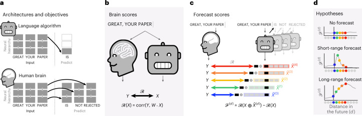
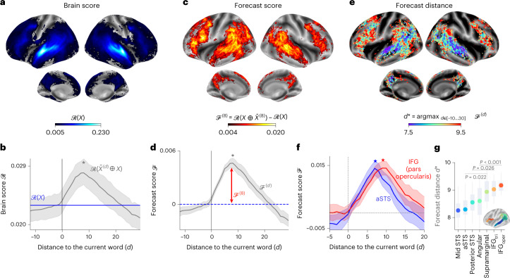
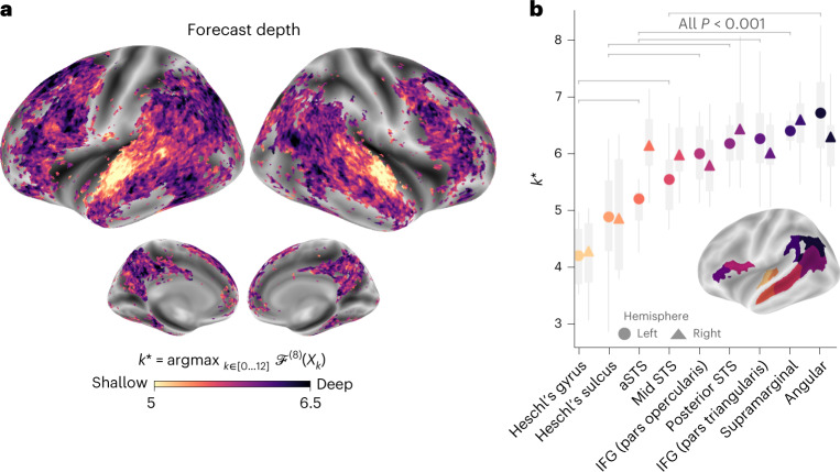
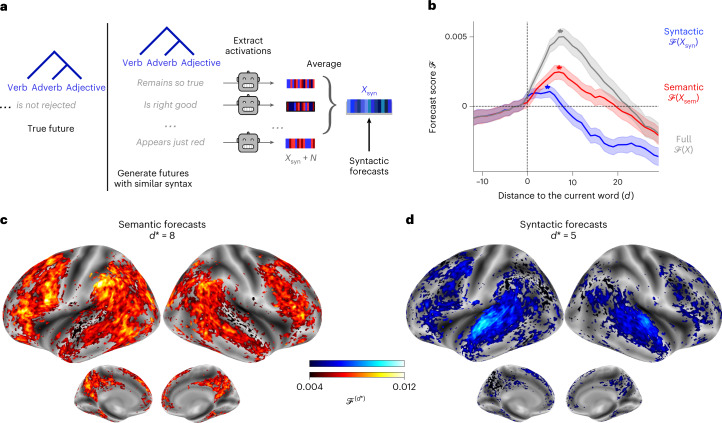
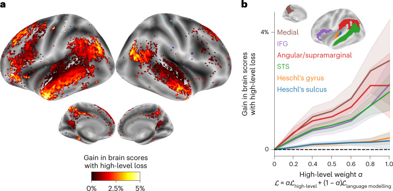
Considerable progress has recently been made in natural language processing: deep learning algorithms are increasingly able to generate, summarize, translate and classify texts. Yet, these language models still fail to match the language abilities of humans. Predictive coding theory offers a tentative explanation to this discrepancy: while language models are optimized to predict nearby words, the human brain would continuously predict a hierarchy of representations that spans multiple timescales. To test this hypothesis, we analysed the functional magnetic resonance imaging brain signals of 304 participants listening to short stories. First, we confirmed that the activations of modern language models linearly map onto the brain responses to speech. Second, we showed that enhancing these algorithms with predictions that span multiple timescales improves this brain mapping. Finally, we showed that these predictions are organized hierarchically: frontoparietal cortices predict higher-level, longer-range and more contextual representations than temporal cortices. Overall, these results strengthen the role of hierarchical predictive coding in language processing and illustrate how the synergy between neuroscience and artificial intelligence can unravel the computational bases of human cognition.

Fig. 1. Experimental approach.

a, Deep language algorithms are typically trained to predict words from their close contexts. Unlike these algorithms, the brain makes, according to predictive coding theory, (1) long-range and (2) hierarchical predictions. b, To test this hypothesis, we first extracted the fMRI signals of 304 individuals each listening to ≈26 min of short stories (Y) as well as the activations of a deep language algorithm (X) input with the same stories. We then quantified the similarity between X and Y with a ‘brain score’: a Pearson correlation $\mathcal{R}$ after an optimal linear projection W (Methods). c, To test whether adding representations of future words (or predicted words; Supplementary Fig. 4) improves this correlation, we concatenated (⊕) the network’s activations (X, depicted here as a black rectangle) to the activations of a ‘forecast window’ ($\tilde{X}$, depicted here as a coloured rectangle). We used PCA to reduce the dimensionality of the forecast window down to the dimensionality of X. Finally, $\mathcal{F}$ quantifies the gain of brain score obtained by enhancing the activations of the language algorithm to this forecast window. We repeated this analysis with variably distant windows (d, Methods). d, Top, a flat forecast score across distances indicates that forecast representations do not make the algorithm more similar to the brain. Bottom, by contrast, a forecast score peaking at d > 1 would indicate that the model lacks brain-like forecast. The peak of ${\mathcal{F}}^d$ indicates how far off in the future the algorithm would need to forecast representations to be most similar to the brain.

Fig. 2. Isolating language predictions and their temporal scope in the human brain.

a, The ‘brain score’ ($\mathcal{R}$; Fig. 1b and Methods), obtained with GPT-2, for each individual and each voxel, here averaged across individuals (n = 304). Only the voxels with significant brain scores are colour-coded. b, Average (across voxels) brain scores obtained with GPT-2 with (grey) or without (blue) forecast representations. The average brain score peaks at d^* = 8 (grey star). c, For each voxel, the average (across individuals) ‘forecast score’ ${\mathcal{F}}^d$, that is, the gain in brain score when concatenating the activations of GPT-2 with a forecast window ${\tilde{X}}^{\left(8\right)}$ is shown. Only the voxels with significant forecast scores are colour-coded. d, Average (across voxels) forecast scores for different distance d. e, Distance that maximizes ${\mathcal{F}}^d$, computed for each individual and each voxel and denoted d^*. This ‘forecast distance’ reveals the regions associated with short- and long-range forecasts. Regions in red and blue are associated with long-range and short-range forecasts, respectively. We only display the voxels with a significant average peak (${\mathcal{F}}^{d^{*}}-{\mathcal{F}}^0,d^{*}=8$; Methods). f, Forecast score within two regions of interest. For each region, we report the average forecast scores of individuals with a representative peak (individuals whose peak belongs to the 45–55 percentiles of all peaks, n = 30 individuals). g, Forecast distance of seven regions of interest, computed for each voxel of each individual and then averaged within the selected brain regions. For all panels, we report the average effect across individuals (n = 304), with the 95% CIs across individuals (b,d,f). P values were assessed with a two-sided Wilcoxon signed-rank test across individuals. In a,c,e, P values were corrected for multiple comparisons across voxels using the FDR and brain maps are thresholded at P < 0.01. The boxplot in g summarizes the distribution of the effect obtained on ten distinct and random subdivisions of the dataset.

Fig. 3. Organization of hierarchical predictions in the brain.

a, Depth of the representation that maximizes the forecast score in the brain, denoted k^*. Forecast scores were computed for each depth, individual and voxel, at a fixed distance of d^* = 8 and averaged across individuals. We computed the optimal depth for each individual and voxel and plotted the average forecast depth across individuals. Dark regions are best accounted for by deep forecasts, while light regions are best accounted for by shallow forecasts. Only significant voxels are colour-coded as in Fig. 2c). b, Same as a but with k^* averaged across the voxels of nine regions of interest, in the left (circle) and right (triangle) hemispheres. Scores were averaged across individuals (n = 304) and the boxplot summarizes the distribution of the effect obtained on ten distinct and random subdivisions of the dataset. Pairwise significance between regions was assessed using a two-sided Wilcoxon rank-sum test on the left hemisphere’s scores (the grey bars indicate P < 0.001).

Fig. 4. Factorizing syntactic and semantic predictions in the brain.

a, Method to extract syntactic and semantic forecast representations, adapted from Caucheteux et al.. For each word and its context (for example, ‘Great, your paper ... ’, we generated ten possible futures with the same syntax as the original sentence (part of speech and dependency tree) but randomly sampled semantics (for example, ‘... remains so true’, ‘... appears so small’). Then, we extracted the corresponding GPT-2 activations (layer eight). Finally, we averaged the activations across the ten futures. This method allowed us to extract the syntactic component common to the ten futures, denoted X_syn. The semantic component was defined as the residuals of syntax in the full activations; X_sem = X − X_syn. We built the syntactic and semantic forecast windows by concatenating the syntactic and semantic components of seven consecutive future words, respectively (Methods). b, Syntactic (blue) and semantic (red) forecast scores, on average across all voxels, as in Fig. 2c. Scores were averaged across individuals; the shaded regions indicate the 95% CIs across individuals (n = 304). The average peaks across individuals are indicated with a star. c, Semantic forecast scores for each voxel, averaged across individuals and at d^* = 8, the distance that maximizes the semantic forecast scores in b. Only significant voxels are displayed as in Fig. 2c. d, Same as c for syntactic forecast scores and d^* = 5.

Fig. 5. Gain in brain score when fine-tuning GPT-2 with a mixture of language modelling and high-level prediction.

a, Gain in brain scores between GPT-2 fine-tuned with language modelling plus high-level prediction (for α_{high level} = 0.5) and GPT-2 fine-tuned with language modelling alone. Only the voxels with a significant gain are displayed (P < 0.05 with a two-sided Wilcoxon rank-sum test after FDR correction for multiple comparisons). b, Brain score gain as a function of the high-level weight α in the loss (equation (8)), from full language modelling (left, α = 0) to full high-level prediction (right, α = 1). Gains were averaged across voxels within six regions of interests (see Methods for the parcellation and Supplementary Fig. 7 for the other regions in the brain). Scores were averaged across individuals and we display the 95% CIs across individuals (n = 304).

References

1. Vaswani, A. et al. Attention is all you need. In Advances in Neural Information Processing Systems, Vol. 30 (Curran Associates, 2017).
1. Radford, A. et al. Language models are unsupervised multitask Learners (2019).
1. Brown, T. B. et al. Language models are few-shot learners. In Advances in Neural Information Processing Systems, Vol. 33, 1877-1901 (Curran Associates, 2020).
1. Fan, A., Lewis, M. and Dauphin, Y. Hierarchical Neural Story Generation. In Proceedings of the 56th Annual Meeting of the Association for Computational Linguistics (Volume 1: Long Papers), 889–898 (Association for Computational Linguistics, 2018).
1. Jain, S. and Huth, A. G. Incorporating context into language encoding models for fMRI. In Proc. 32nd Conference on Neural Information Processing Systems (NeurIPS 2018), Vol. 31, (Curran Associates, 2018).
Publication types