Validation of thermal dynamics during Hyperthermic IntraPEritoneal Chemotherapy simulations using a 3D-printed phantom

Abstract

Introduction: CytoReductive Surgery (CRS) followed by Hyperthermic IntraPeritoneal Chemotherapy (HIPEC) is an often used strategy in treating patients diagnosed with peritoneal metastasis (PM) originating from various origins such as gastric, colorectal and ovarian. During HIPEC treatments, a heated chemotherapeutic solution is circulated through the abdomen using several inflow and outflow catheters. Due to the complex geometry and large peritoneal volume, thermal heterogeneities can occur resulting in an unequal treatment of the peritoneal surface. This can increase the risk of recurrent disease after treatment. The OpenFoam-based treatment planning software that we developed can help understand and map these heterogeneities.

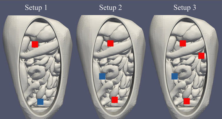
Methods: In this study, we validated the thermal module of the treatment planning software with an anatomically correct 3D-printed phantom of a female peritoneum. This phantom is used in an experimental HIPEC setup in which we varied catheter positions, flow rate and inflow temperatures. In total, we considered 7 different cases. We measured the thermal distribution in 9 different regions with a total of 63 measurement points. The duration of the experiment was 30 minutes, with measurement intervals of 5 seconds.

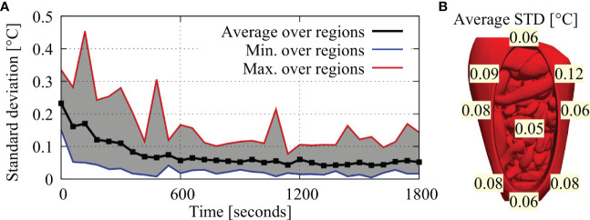
Results: Experimental data were compared to simulated thermal distributions to determine the accuracy of the software. The thermal distribution per region compared well with the simulated temperature ranges. For all cases, the absolute error was well below 0.5°C near steady-state situations and around 0.5°C, for the entire duration of the experiment.

Discussion: Considering clinical data, an accuracy below 0.5°C is adequate to provide estimates of variations in local treatment temperatures and to help optimize HIPEC treatments.

Keywords: cancer biology; computational fluid dynamics (CFD); computational modeling; hyperthermic intrapertioneal chemotherapy (HIPEC); translational research; treatment planning software; validation.

Figure 1

The 3D design of the phantom (A) and the 3D-printed phantom based on the design in A (B). The oval opening of the peritoneal cavity (see label abdominal opening) mimics a “Colosseum” setup, often used during an open HIPEC treatment. Panel (C) shows a photograph of the phantom during experimentation. Schematic diagram of the setup used during experiments (D). A roller pump (1) circulates water from the outflow (2) through two heat exchangers (3) placed inside water baths and back into the phantom (4). Temperatures are measured in 9 different regions (5) using 9 7-point thermocouple probes. The thermometry system (6) records temperatures which are monitored and stored on a PC (7). In panel (E) we visualize the location of the various probe regions used for evaluation of thermal profiles. Panels (F–H) show photographs of the roller pump, catheter tips locked in position and heat exchanger, respectively.

Figure 2

Visualization of the catheter setups used in this study. From left to right we show the positions for the 1 inflow/1 outflow, 2 inflow/1 outflow and 3 inflow/1 outflow cases, respectively. Inflows are visualized in red, the outflow in blue. For setup 1, the inflow was positioned near the liver and the outflow was positioned near the rectum. For setup 2, inflows were positioned near the liver and rectum and the outflow was positioned slightly right to the patient’s center to allow the catheter tips to be at a depth of 3 cm. For setup 3, inflows were positioned near the liver, descending colon and rectum and the outflow was positioned slightly right to the patient’s center.

Figure 3

Visualization of the computational geometry used during simulations. In total, 5 boundaries were defined: inflow and outflow patch (pink and orange, respectively), peritoneal exterior to the surroundings (red), peritoneal interior to the peritoneal exterior (white) and the peritoneal interior to the surroundings (blue).

Figure 4

(A) Minimum, maximum and average standard deviations over all regions, plotted over time. Standard deviations are highest near the start of the experiment and decrease towards a steady-state near the end of the experiment. (B) Average standard deviations per region.

Figure 5

Comparison of measurements and predicted thermal ranges for the baseline setup (case # 1). (A-I) shows the comparison for region 1-9, with the locations of these regions shown in (J). Simulated averages and ranges are represented by the black lines and shaded areas and measurements are represented by the colored dots. Measurements were taken every 5 seconds, with probes featuring 7 measurement points per probe. Therefore, each plot shows 2520 measurements over the duration of the experiment. In general, measurements fall within the predicted ranges, especially near steady state (last 5 minutes).

Figure 6

Effect of the flow rate on the temperature in each region and on the outflow temperature. In figure (A, B), average values for region 1 through 5 and 6 through 9 plus outflow are plotted for three different flow rates (600, 800 and 1000 mL/min),respectively. The values shown are calculated as the average over the last 5 minutes of the predicted (colored line) or measured values (min/max values in that last five minutes shown by the whiskers and the average shown by the symbols). All regions show an increase in treatment temperature after 25 minutes, correctly predicted by simulated profiles.

Figure 7

Visualization of the simulated thermal distributions and the effect of changes in flow rate on the distribution. White squares denote the location of the inflow catheter and temperatures below 39°C are black. The thermal distribution of case #1 (A) shows that a high flow rate at one location results in high temperatures near the inflow and surroundings. Reducing the flow rate to 800 mL/min (B) and 600 mL/min (C) results in lower temperatures, most notably in distant regions.

Figure 8

Web diagram showing the average steady state temperature for different inflow temperatures. Measured temperatures are visualized by a ■ , ▲ and • for inflow temperatures of 37.7°C, 42.7°C and 47.7°C, respectively. Simulated temperatures are represented by a blue, orange and red lines for inflow temperatures of 37.7°C, 42.7°C and 47.7°C, respectively. Similar distributions are visible for all inflow temperatures. Region 1, 4, 5 and the outflow are all close to the inflow temperature while region 2, 3 and 6 are well below the inflow temperature. Ideally, all temperatures would approach their respective upper levels, e.g. 37°C, 42 text degree C and 47°C.

Figure 9

Visualization of the simulated thermal distributions and the effect of changes in catheter setup on the distribution. White squares denote the location of the inflow catheter, white circles denote the location of the outflow catheter and temperatures below 39°C are black. The thermal distribution of case #1 (A) shows that using one inflow at high flow rate results in high temperatures near the inflow and surroundings. Addition of 1 (B) or 2 (C) extra inflow catheters results in a more homogeneous overall distribution.

References

-
- Privalov A, Vazenin A, Chernova L, Taratonov A, Gubaydulina T. Ovarian cancer with peritoneal carcinomatosis: Comparing of photodynamic treatment and hipec. J Clin Oncol (2017) 35:e17040–0. doi: 10.1200/JCO.2017.35.15_suppl.e17040 - DOI
- Verwaal VJ, van Ruth S, de Bree E, van Slooten GW, van Tinteren H, Boot H, et al. . Randomized trial of cytoreduction and hyperthermic intraperitoneal chemotherapy versus systemic chemotherapy and palliative surgery in patients with peritoneal carcinomatosis of colorectal cancer. J Clin Oncol (2003) 21:3737–43. doi: 10.1200/JCO.2003.04.187 - DOI - PubMed
LinkOut - more resources
Full Text Sources
Miscellaneous