Identifying regulation with adversarial surrogates

Abstract

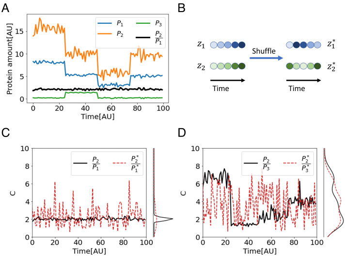
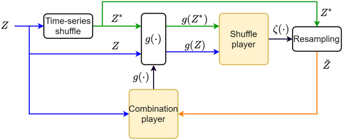
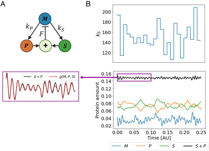
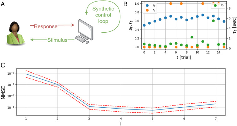
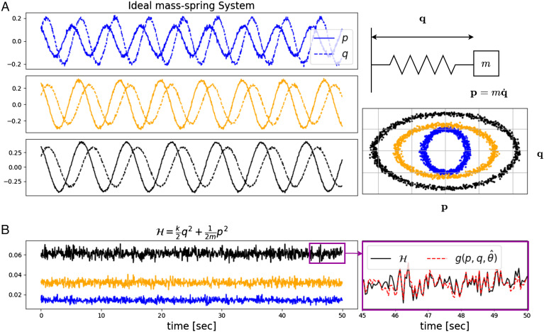
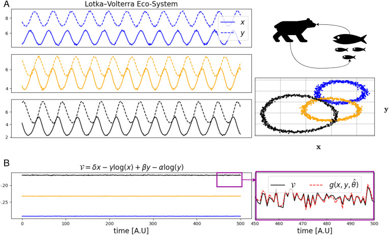
Homeostasis, the ability to maintain a relatively constant internal environment in the face of perturbations, is a hallmark of biological systems. It is believed that this constancy is achieved through multiple internal regulation and control processes. Given observations of a system, or even a detailed model of one, it is both valuable and extremely challenging to extract the control objectives of the homeostatic mechanisms. In this work, we develop a robust data-driven method to identify these objectives, namely to understand: "what does the system care about?". We propose an algorithm, Identifying Regulation with Adversarial Surrogates (IRAS), that receives an array of temporal measurements of the system and outputs a candidate for the control objective, expressed as a combination of observed variables. IRAS is an iterative algorithm consisting of two competing players. The first player, realized by an artificial deep neural network, aims to minimize a measure of invariance we refer to as the coefficient of regulation. The second player aims to render the task of the first player more difficult by forcing it to extract information about the temporal structure of the data, which is absent from similar "surrogate" data. We test the algorithm on four synthetic and one natural data set, demonstrating excellent empirical results. Interestingly, our approach can also be used to extract conserved quantities, e.g., energy and momentum, in purely physical systems, as we demonstrate empirically.

Keywords: artificial neural networks; biological control; biological regulation; computational biology; data analysis.

Fig. 1.

Coefficient of Regulation (CR) as a measure of combination invariance. (A) A synthetic example of ratio control in a biological system. The amounts of three proteins, P₁, P₂, and P₃, fluctuate over time and are modulated by discontinuous perturbations (t​ = ​25, 50, 75). In the face of these perturbations, the ratio $\raisebox{1ex}{$P_2(t)$}\!\left/ \!\raisebox{-1ex}{$P_1(t)$}\right.$ is held around a setpoint c_set​ = ​2 with small fluctuations (noise with SD 0.15). (B) To calculate CR, temporal correlations between the measurements are destroyed by shuffling the time points of each measurement independently. (C) While the distribution of $\raisebox{1ex}{$P_2(t)$}\!\left/ \!\raisebox{-1ex}{$P_1(t)$}\right.$ in real data is narrow (black), the distribution of the ratio between shuffled measurements is much wider (red dashed), resulting in a small CR. (D) Since there is no correlation between P₂ and P₃, the distributions of their ratio in real and in shuffled data are of the same width, and CR = 1.

Fig. 2.

Failure of straightforward optimization. Optimal combination values found by the single-player algorithm, a neural network which minimizes the Coefficient of Regulation with unconstrained shuffling (CR, Eq. 5, ζ(⋅)≡1). This algorithm was fed with time traces of the three proteins, with the ratio $\raisebox{1ex}{$P_2$}\!\left/ \!\raisebox{-1ex}{$P_1$}\right.$ being the conserved combination. The network output is displayed as an arbitrary-value colormap in the (P₁, P₂) plane. Shuffles that fall within the boundaries of the data (the white lines) have a practically fixed value, while shuffles outside these boundaries attain values that are correlated with their distance from the boundaries. The found combination has a CR of almost zero (0.004 ± 0.003). However, its Pearson correlation with the ground truth conserved combination is 0.11 ± 0.08.

Fig. 3.

IRAS Algorithm outline. The time-series data Z is shuffled to create the unconstrained shuffled time-series Z^*. The “shuffle player,” exposed only to the 1D combinations g(Z) and g(Z^*), sets the weighting function ζ(⋅) used to resample $\tilde{Z}$ from Z^*, such that the 1D distributions, P_Z(g(Z)) and $P_{\tilde{Z}}(g(\tilde{Z}))$, are identical. Then, given Z and $\tilde{Z}$, the “combination player” updates g(⋅) toward minimizing its CR. These steps continue to iterate until no further improvement is possible.

Fig. 4.

IRAS demonstration. (A) A step of the iterative algorithm (Fig. 3) is displayed. Top Left: the value of an intermediate combination g(⋅) given by the combination player, is displayed in the (P₁, P₂) plane together with the true combination (red line) and the data limits (white lines). Top Right: distriubtions of this combination over the data (P_Z(g(Z)), blue) and unconstrained shuffles (P_Z^*(g(Z^*)), dashed green). Bottom Right: The shuffle player examines these 1D distributions and resamples Z^* via the weighting function ζ(⋅) to construct the constrained shuffles $\tilde{Z}$, over which the 1D distribution of g matches the data. The resampling probability is displayed in the (P₁, P₂) plane. Bottom Left: Combination player receives this resampled shuffled ensemble, another optimization step begins and the combination player updates g(⋅). (B) Combination values (Top Left) and resample probability (Top Right) at the final iteration. The combination player has captured the control objective (the map approximates $\raisebox{1ex}{$P_2$}\!\left/ \!\raisebox{-1ex}{$P_1$}\right.$), and the shuffle player has captured the data distribution (delineated by white lines). Bottom: values of the combination along a stretch of time together with the ground-truth combination.

Fig. 5.

IRAS captures the control objective in a kinetic model. (A) An illustration of the closed loop system. Protein M induces the production of both S and P and receives a negative feedback of their sum. (B) Top: perturbations cause step-like variation in k_S over time. The duration of each step is 0.01 which is much longer than the timescale of the feedback loop $\tau =\raisebox{1ex}{$1$}\!\left/ \!\raisebox{-1ex}{$F$}\right.=0.0005$ (F = 2, 000). This enables the controller to track the changes in S + P. Each step was sampled from a normal distribution with a mean 150 and a SD 30. The rest of the parameters were sampled similarly: γ_P, γ_S = 70 ± 15, γ_M = 80 ± 15, k_P = 150 ± 30. Bottom Right: The trajectories of the three proteins and the combination S + P over time. The Bottom Left: a zoom-in of the combination P + S (black) within the purple box in the Right panel along with the output of the algorithm (dashed red).

Fig. 6.

Relational dynamics in perception (A) Trial-trial variability in human sensory detection is tested. A synthetic feedback controller sets the stimulus, which is the contrast of a foreground raster displayed on the screen. Then, the user responds positively when detecting the raster or negatively when not. (B) Raw data from psychophysics experiment. A portion of the measured time-series z_t = [s_t r_t τ_t] in a human sensory detection experiment. The stimulus s_t (blue dots) is a time-series of image-contrast values, the responses r_t (orange dots) are a Boolean time-series of detection, and τ_t (green dots) is the reaction time from stimulus to response. (C) Normalized mean-square-errors of stimulus estimation values as defined in Eq. 16. Stimulus estimation is obtained from the analytical expression of the feedback loop detected. The estimation errors decrease monotonously up to T = 5 implying an effective timescale of 5 trials. Dashed red lines are the MSE of errors higher and lower than the MSE which lies on the blue line.

Fig. 7.

IRAS captures the conservation law in Hamiltonian mechanics. The dataset contains 100 different mass-spring systems. In each system, k and m were sampled uniformly between [0.5, 1.5] and the initial conditions, p₀ and q₀ between [0.15, 0.25] and [0.1, 0.2] respectively. The raw observations consist of times-series of length 1,000 of p and q corrupted by a zero-mean additive Gaussian white noise with SD 0.01. (A) Top Right: ideal mass on spring with mass m and spring constant k. Left: time traces of momentum, (p, solid lines) and coordinate, (q, dashed lines) for ideal mass–spring systems with spring and mass constants k = (0.72, 1.13, 1.05) and m = (0.59, 1.32, 1.48) in the Top, Middle, and Bottom panels, respectively. Bottom Right: same trajectories plotted in the phase plane (p, q). (B) Left: the energy as a function of time for the three systems in (A) with corresponding colors. Right: a zoom-in of the energy and output of the combination learned by IRAS in a short stretch of time.

Fig. 8.

IRAS captures the conservation law in predator–prey dynamical systems. The dataset contains 100 systems where in each system, the parameters were sampled uniformly within a range of 0.1 about the values (α, β, γ, δ)=(0.25, 0.075, 0.15, 0.07), and the initial conditions, x₀ and y₀ within a range of 1.0 about the values (x₀, y₀)=(4.5, 7.5). The raw observations consist of times-series of length 500 of x and y corrupted by a zero-mean Gaussian white noise with SD 0.055. (A) Top Right: predator–prey illustration. Left: time traces of the numbers of predator, (x, solid lines) and prey, (y, dashed lines) for a Lotka–Volterra model with parameters α = (0.208, 0.205, 0.200), β = (0.026, 0.032, 0.034), γ = (0.106, 0.106, 0.101) and δ = (0.020, 0.021, 0.028) in the Top, Middle, and Bottom panels, respectively. Bottom Right: same trajectories plotted in the phase plane (x, y). (B) Left: the conserved quantity as a function of time for the three systems in (A) with corresponding colors. Right: zoom of the conserved quantity and output of the combination learned by IRAS in a short stretch of time.

References

1. G. E. Billman, Homeostasis: The underappreciated and far too often ignored central organizing principle of physiology. Front. Physiol. 11, 200 (2020). - PMC - PubMed
1. Hsiao V., Swaminathan A., Murray R. M., Control theory for synthetic biology: Recent advances in system characterization, control design, and controller implementation for synthetic biology. IEEE Control Syst. Magaz. 38, 32–62 (2018).
1. Kotas M. E., Medzhitov R., Homeostasis, inflammation, and disease susceptibility. Cell 160, 816–827 (2015). - PMC - PubMed
1. El-Samad H., Biological feedback control-respect the loops. Cell Syst. 12, 477–487 (2021). - PubMed
1. A. Stawsky, H. Vashistha, H. Salman, N. Brenner, Multiple timescales in bacterial growth homeostasis. Iscience 25, 103678 (2022). 10.1016/j.isci.2021.103678. - DOI - PMC - PubMed
Publication types
LinkOut - more resources