Fast and sensitive GCaMP calcium indicators for imaging neural populations

Abstract

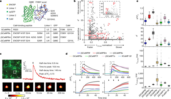
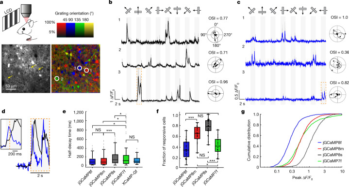
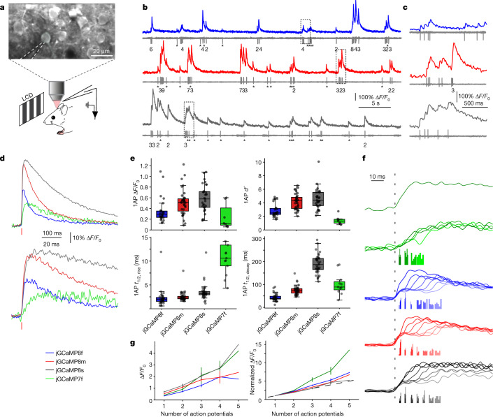
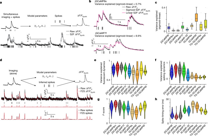
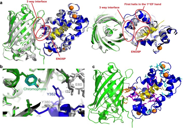
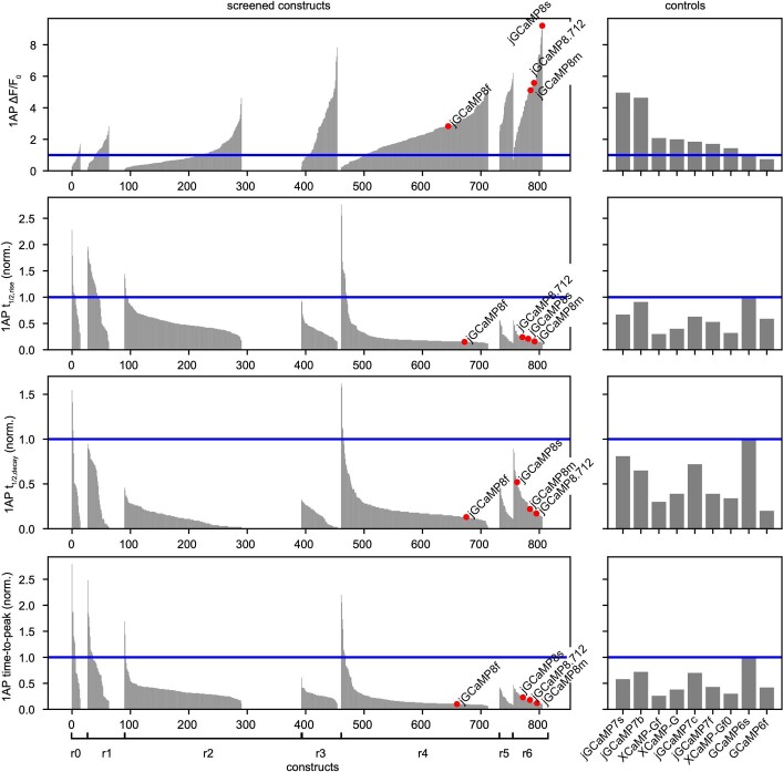
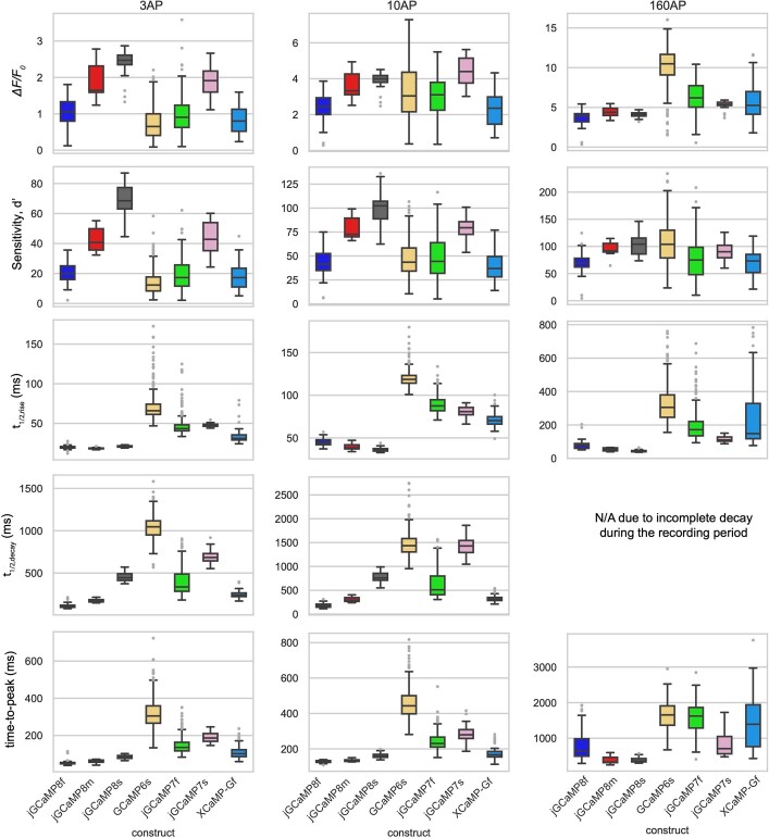
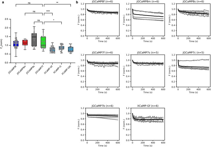
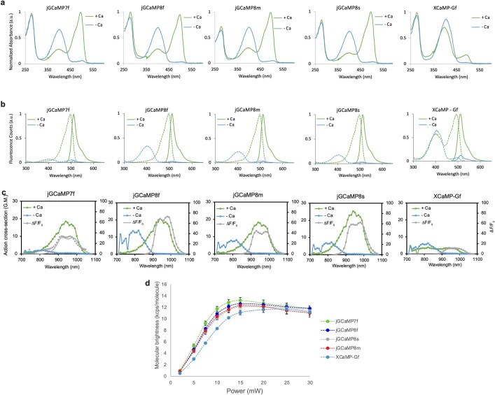
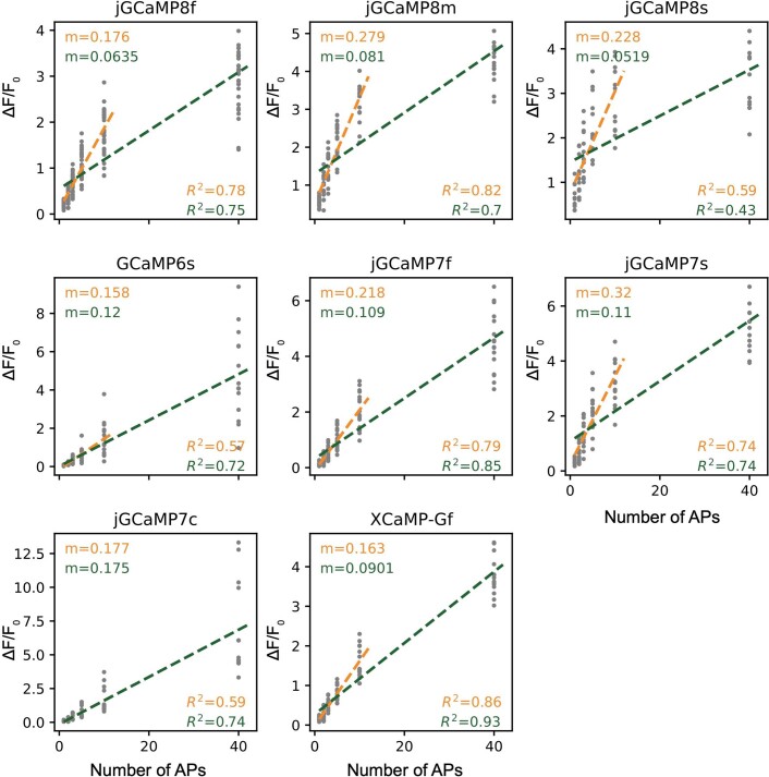
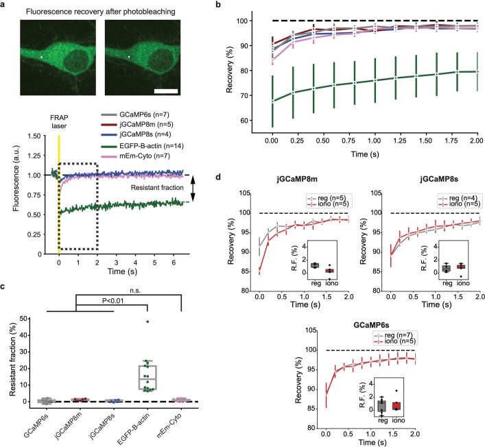
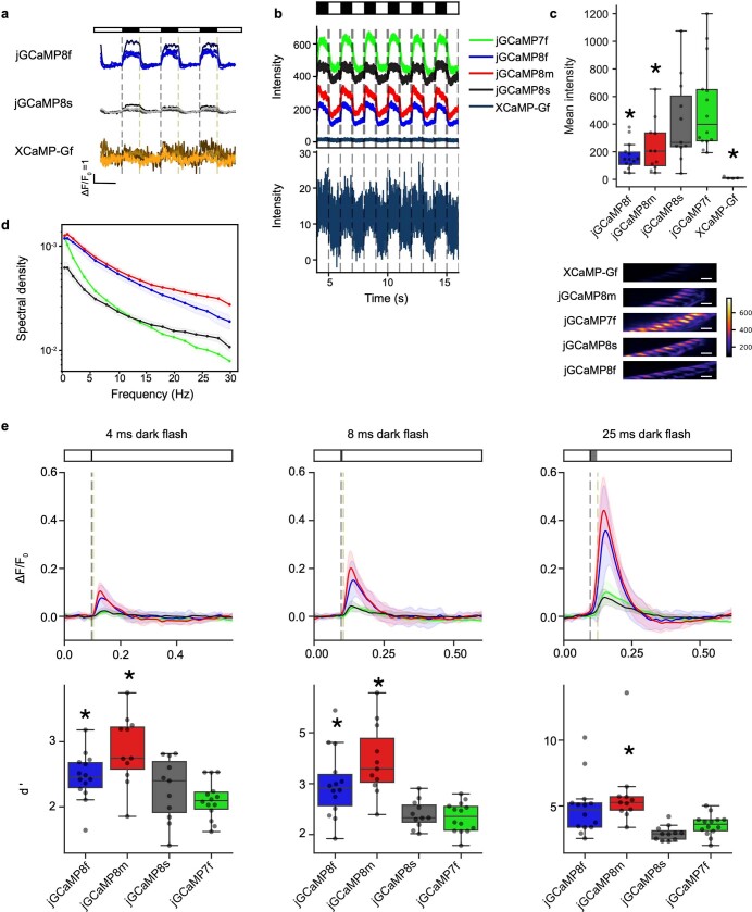
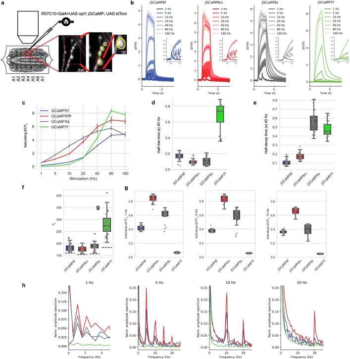
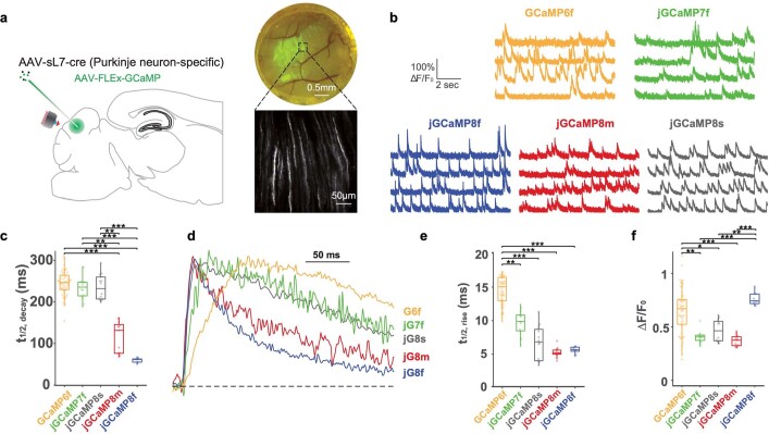
Calcium imaging with protein-based indicators^1,2 is widely used to follow neural activity in intact nervous systems, but current protein sensors report neural activity at timescales much slower than electrical signalling and are limited by trade-offs between sensitivity and kinetics. Here we used large-scale screening and structure-guided mutagenesis to develop and optimize several fast and sensitive GCaMP-type indicators^3-8. The resulting 'jGCaMP8' sensors, based on the calcium-binding protein calmodulin and a fragment of endothelial nitric oxide synthase, have ultra-fast kinetics (half-rise times of 2 ms) and the highest sensitivity for neural activity reported for a protein-based calcium sensor. jGCaMP8 sensors will allow tracking of large populations of neurons on timescales relevant to neural computation.

Fig. 1. GCaMP mutagenesis and screening in neuronal culture.

a, jGCaMP8 (variant 8.410.80) structure and mutations in different jGCaMP8 variants relative to GCaMP6s (top). ENOSP, linker 1 (ENOSP–cpGFP), linker 2 (cpGFP–CaM), cpGFP, CaM, mutated sites (red) and Ca²⁺ ions (orange) are shown. Mutations for each jGCaMP8 variant (bottom table) are also displayed. b, Sensitivity (d′) and rise kinetics (t_1/2,rise) for jGCaMP8 variants. The x axis is normalized to GCaMP6s. GCaMP6, jGCaMP7, jGCaMP8 and XCaMP are highlighted in red. Mutants with normalized t_1/2,rise > 1.1 are not shown. The inset shows a zoomed in view on the jGCaMP8 series. Complete multi-parameter scatterplots are available as an interactive Binder notebook (Methods). c, Screening in neurons. Field stimulation of jGCaMP8m-expressing cultured neurons (top left), a fluorescence trace (1AP) (top right) and single frames of F corresponding to the box in the image (bottom) are shown. Scale bar, 100 µm. d, Responses to 1AP (black bar; top left) and 3AP (black bars; top right). Zoomed-in insets from the top panel (dashed boxes) to highlight rise kinetics are also shown (bottom). Solid lines indicate the mean and the shaded area denotes s.e.m. (n = 48 wells and 1,696 neurons (jGCaMP8f), n = 11 wells and 496 neurons (jGCaMP8m), n = 24 wells and 1,183 neurons (jGCaMP8s), n = 283 wells and 8,700 neurons (GCaMP6s), n = 294 wells and 7,372 neurons (jGCaMP7f), n = 22 wells and 514 neurons (jGCaMP7s), and n = 69 wells and 1,305 neurons (XCaMP-Gf); overall statistics, n = 7 independent transfections, 38 96-well plates). Data shown represent a portion of the overall screened constructs in Supplementary Table 1. e, Responses to 1AP for jGCaMP8 indicators and comparison with GCaMP6s, jGCaMP7f, jGCaMP7s and XCaMP-Gf. Data and n values are the same as in d. For the box-and-whisker plots, the box indicates the median and 25–75th percentile range, and the whiskers indicate the shorter of 1.5 times the interquartile range or the extreme data point.

Fig. 2. jGCaMP8 performance in Drosophila.

a, Schematic of the experiment. Fly with visual stimulus (top), fluorescence micrograph of L2 dendrites in medullar layer 2 (scale bar, 5 μm) (middle), and a schematic of the Drosophila visual system (bottom) are shown. b, ΔF/F₀ response to a 0.5-Hz visual stimulation frequency from variants jGCaMP7f and jGCaMP8m. Individual traces show four representative individual animals per GECI (shading arbitrary). Light and dark periods are indicated by white and black bars above the graph. The error bands represent s.e.m. c, Mean ΔF/F₀ response to 0.5-Hz stimulation. The solid line indicates the mean and the shaded area denotes s.e.m. The dark period is represented by a black bar above the graph. The mean was calculated from eight trials per animal and then between animals. The inset compares the response from each variant at the onset of the dark period. d, Half-rise and half-decay times for responses in c. Half-rise: 128 ± 11 ms (jGCaMP7f), 76 ± 8 ms (jGCaMP8f), 58 ± 6 ms (jGCaMP8m) and 80 ± 8 ms (jGCaMP8s) (Kruskal–Wallis multiple-comparison test, P = 2.9 × 10⁻⁴; pairwise Dunn’s comparison test with jGCaMP7f: P = 3.1 × 10⁻³ (jGCaMP8f), P = 2.9 × 10⁻⁵ (jGCaMP8m) and P = 1.3 × 10⁻² (jGCaMP8s)). Half-decay times: 277 ± 29 ms (jGCaMP7f), 192 ± 26 ms (jGCaMP8f), 137 ± 21 ms (jGCaMP8m) and 198 ± 21 ms (jGCaMP8s) (Kruskal–Wallis multiple-comparison test, P = 2.4 × 10⁻²; pairwise Dunn’s comparison test: P = 1.1 × 10⁻¹ (jGCaMP8f), P = 2.2 × 10⁻³ (jGCaMP8m) and P = 1.8 × 10⁻¹ (jGCaMP8s)). *P < 0.05. Total n of flies tested for each variant in c and d: 14 (jGCaMP7f), 11 (jGCaMP8s), 11 (jGCaMP8m) and 14 (jGCaMP8f). For the box-and-whisker plots, the box indicates the median and 25–75th percentile range, and the whiskers indicate the shorter of 1.5 times the interquartile range or the extreme data point.

Fig. 3. Imaging neural population in the mouse V1 in vivo.

a, Schematic of the experiment (top left). Example image of V1 L2/3 cells (three cells marked by yellow arrows) expressing jGCaMP8s (bottom left), and the same field of view (FOV) colour-coded (three corresponding cells circled) based on the preferred orientation of the neuron (hue) and response amplitude (brightness) (bottom right with colour coding above). This experiment was repeated independently with similar results in 26 FOVs from 6 mice. b,c, Example traces from three L2/3 neurons expressing jGCaMP8s (b; same cells as indicated in a) or jGCaMP8f (c). Averages of five trials with shaded s.e.m. The polar plots indicate the preferred direction of cells. The orientation selectivity index (OSI) is displayed above each polar plot. d, Example zoomed-in fluorescence traces corresponding to the orange boxes in b (jGCaMP8s in black) and c (jGCaMP8f in blue), normalized to the peak of the response. The inset shows additional detail of the first transient. e, Half-decay time of the fluorescence response after the end of the visual stimulus (n = 320 cells from 3 mice (jGCaMP7f), 124 cells from 3 mice (XCaMP-Gf), 317 cells from 5 mice (jGCaMP8f), 365 cells from 3 mice (jGCaMP8m) and 655 cells from 6 mice (jGCaMP8s)). Kruskal–Wallis multiple-comparison test: P < 0.001. Dunn’s comparison test: *P < 0.05, ***P < 0.001 and not significant (NS). Full statistics are in the Methods. f, Proportion of cells responding to visual stimuli (n = 12 FOVs from 3 mice (jGCaMP7f), 19 FOVs from 5 mice (jGCaMP8f), 14 FOVs from 3 mice (jGCaMP8m) and 26 FOVs from 6 mice (jGCaMP8s)). Tukey’s multiple-comparison test: P < 0.001. One-way ANOVA test was used: *P < 0.05, ***P < 0.001 and NS. Full statistics are in the Methods. g, Distribution of response amplitude (ΔF/F₀) for preferred stimulus. The 75th percentile ΔF/F₀ values for each construct: 98% (jGCaMP7f), 38% (jGCaMP8f), 83% (jGCaMP8m) and 183% (jGCaMP8s). n = 1,053 cells from 3 mice (jGCaMP7f), 1,253 cells from 5 mice (jGCaMP8f), 848 cells from 3 mice (jGCaMP8m) and 1,026 cells from 6 mice (jGCaMP8s). Full statistics are in the Methods.

Fig. 4. Simultaneous electrophysiology and imaging in the mouse V1 in vivo.

a, Schematic of the experiment. Representative FOV (top) is also shown. The recording pipette is indicated by dashed lines. b, Simultaneous fluorescence and spikes, for example, neurons expressing jGCaMP8f (top), jGCaMP8m (middle) and jGCaMP8s (bottom). The number of spikes for each burst is indicated below the trace (single spikes are indicated by asterisks). c, Zoomed-in view of traces corresponding to the dashed boxes in b. d, Grand average of fluorescence response elicited by single APs, aligned to the AP peak (red vertical bar), reconstructed at a temporal resolution of 500 Hz (see text and Extended Data Fig. 15 for details). e, Properties of fluorescence responses elicited by single APs. The dots indicate single cells. For the box-and-whisker plots, the box indicates the median and 25–75th percentile range, and whiskers indicate the shorter of 1.5 times the interquartile range or the extreme data point. n = 24 cells from 9 mice (jGCaMP8f), 35 cells from 11 mice (jGCaMP8m), 31 cells from 10 mice (jGCaMP8s) and 11 cells from 3 mice (jGCaMP7f). f, Normalized jGCaMP7f response to a single AP (from d) (top), and response to AP doublets, binned based on interspike intervals (bottom). Transient responses are normalized and aligned to the first AP of the doublet (dashed line). The timing of the second AP is represented by the histograms below the transient responses. The interspike intervals are selected to be approximately 5, 10, 15, 20, 25, 30 and 35 ms. Responses for jGCaMP7f (green), jGCaMP8f (blue), jGCaMP8m (red) and jGCaMP8s (black) are shown. g, Response linearity. Peak response as a function of the number of APs within a 20-ms window (left) is shown. Mean and s.e.m. are displayed. The right graph is the same as the graph on the left, but normalized to 1AP response. n = 33, 23, 14, 4 and 2 cells (jGCaMP8f); n = 41, 32, 19, 6 and 2 cells (jGCaMP8m); n = 38, 34, 18, 3 and 1 cells (jGCaMP8s); and n = 15, 13, 6, 4 and 2 cells (jGCaMP7f) for 1, 2, 3, 4 and 5 APs, respectively.

Fig. 5. Spike-to-fluorescence and fluorescence-to-spike models.

a, Spike-to-fluorescence (S2F) model. Schematic plot of the S2F forward model that generates a synthetic fluorescence trace (∆F/F_Synth) from an input spike train (top), and an example fit and data for one cell (bottom) are shown. Measured ∆F/F₀ (black) is overlaid with the simulated ∆F/F_Synth (grey) from the S2F model. The input to the model, the simultaneously recorded spikes (black), are shown below the traces. b, Exemplary cell dynamics with different degrees of non-linearities. c, The degree of non-linearity (measured by the difference of variance explained using a sigmoid fit from that using a linear fit). Non-linearity is low for jGCaMP8 sensors (see Extended Data Table 5 for more details) but high for GCaMP6 sensors (TG: GCaMP6 transgenic mouse; otherwise, AAV application). The minima indicate 0th percentile of data (0%); the maxima denote 100%; the centre line indicates 50%; the bounds of box are from 25% (lower quartile) to 75% (upper quartile); and the whiskers indicate 1.5 times the distance between the upper and lower quartiles. The number of biologically independent cells collected in each condition is shown in Extended Data Table 5. d, Fluorescence-to-spike (F2S) model. Schematic plot of the F2S inference model that generates a synthetic fluorescence trace (∆F/F_Synth) from an inferred spike train (top), and an example fit and data of a cell (bottom) are shown. The first row shows experimental spikes and the measured ∆F/F₀ overlaid with the simulated ∆F/F_Synth from the F2S model. The second row shows the simultaneously recorded ground-truth spikes (black), shown below the traces, compared with the inferred spikes (red). The third row shows the recorded spike rate overlaid with the inferred spike rate from the F2S model. e–h, Violin plots, lines from top to bottom: 75%, 50%, 25% of data, respectively. e,f, Performance of fitting activity using the linear F2S model. Fluorescence dynamics (fits compared with raw fluorescence) (e) and spiking (fits compared with ground-truth spiking dynamics) (f) are shown. g, Performance of spike detectability using the linear F2S model. h, Spike-timing error using the linear F2S model.

Extended Data Fig. 1. Crystal structure of jGCaMP8.410.80.

ENOSP (yellow), linker 1 (ENOSP-cpGFP, grey), linker 2 (cpGFP-CaM, grey), cpGFP (green), CaM (blue), Ca²⁺ ions (orange). a. Overlay of the structures of jGCaMP8.410.80 and GCaMP5G (light grey). Left: side view. Right: top view. b. A closeup of the chromophore region in structures of jGCaMP8.410.80 and GCaMP5G. Ile32 (dark gray) in Linker 1 of jGCaMP8.410.80 facilitates closer interaction of Tyr352 (blue) with the GFP chromophore. The corresponding residues in GCaMP5G, Glu60 and Tyr380, are depicted in light gray. c. Individual residue mutations screened in this study, shown on the structure of jGCaMP8.410.80. Sixteen initial interface positions are in orange. Ten subsequently mutated CaM positions are in magenta. Mutations based on the FGCaMP sensor are in cyan.

Extended Data Fig. 2. Results of cultured neuron 1-AP field stimulation screen (n = 813 constructs, 647 with detectable 1-AP responses; Methods).

All results are normalized to in-plate GCaMP6s controls (blue line) and listed in ranked order (increasing for peak ΔF/F₀, decreasing for all others) from each screening round. Other relevant control constructs (n = 9) were screened side-by-side (right panels). Sensor engineering took place over seven rounds: Round 0 (r0): Graft peptides (n = 29 constructs). Round 1 (r1): Screen linkers (n = 64 constructs). Round 2 (r2): Site-saturation mutagenesis of 16 interface positions: 7 in ENOSP, 4 on cpGFP, and 5 on CaM (n = 304 constructs). Round 3 (r3): Combination of beneficial mutations to date (n = 69 constructs). Round 4 (r4): Site-saturation mutagenesis of 10 additional CaM positions surrounding ENOSP and of 3 residues on linker1 (n = 272 constructs). Graft mutations from FGCaMP. Round 5 (r5) and 6 (r6): Two additional rounds of combination of beneficial mutations (n = 25, 51 constructs respectively).

Extended Data Fig. 3. Response characteristics of jGCaMP8 indicators to 3, 10, and 160 field stimulation pulses (45 V, 83 Hz).

Half-decay at 160 pulses is not reported because cell fluorescence typically does not decay to baseline during our imaging time (6 s after stimulus onset). n values same as in Fig. 1d,e. Box-whisker plots indicate the median and 25^th–75^th percentile range; whiskers indicate the shorter of 1.5 times the inter-quartile range or the extreme data point.

Extended Data Fig. 4. Baseline brightness and photobleaching of sensors.

a. Baseline brightness. The jGCaMP8 series exhibited similar baseline fluorescence in the cultured neuron assay compared to jGCaMP7f, but XCaMP sensors were significantly dimmer (H(6) = 71.77, P < 0.0001, Kruskal-Wallis test; Dunn’s multiple comparisons test with jGCaMP7f as control). n.s.: not significant (P > 0.99). *P = 0.012; **P = 0.0012; ****P < 0.0001. Each point represents median neuronal brightness from a single well. jGCaMP8f: n = 40, jGCaMP8m: n = 8, jGCaMP8s: n = 18, jGCaMP7f: n = 20, XCaMP-Gf: n = 29, XCaMP-G: n = 31, XCaMP-Gf0: n = 16; overall statistics: n = 2 independent transfections, 5 96-well plates. Box-whisker plots indicate the median and 25^th–75^th percentile range; whiskers indicate the shorter of 1.5 times the inter-quartile range or the extreme data point. b. Photobleaching of jGCaMP8, jGCaMP7, and XCaMP variants in neuron cell culture. Grey lines: individual cells, black lines: mean. Each cell’s fluorescence trace was normalized to the initial value. N values indicate number of cells (n = 1 well per variant, n = 1 transfection day). After continuous illumination for 10 min, neurons transfected with jGCaMP8 variants lost on average 13-28% of their initial fluorescence. jGCaMP8m exhibited biphasic bleaching: a rapid phase consisting of ~15% fluorescence loss within 10 s followed by a slower phase (10% within 10 min). Of the other variants, jGCaMP7c also exhibited this property. We noticed considerable variability in the photobleaching rates within individual neurons, possibly stemming from expression level and differences in baseline brightness in each neuron as a function of intracellular resting [Ca²⁺].

Extended Data Fig. 5. Photophysical characterization of jGCaMP8 sensors.

a. One-photon absorbance spectra of jGCaMP sensors acquired in 10 mM MOPS, pH 7.2. b. One-photon excitation and emission spectra of jGCaMP8 sensors. Emission spectra were calculated with 460 nm excitation light (bandwidth 5 nm); excitation spectra were calculated with 540 nm emission light (bandwidth 5 nm). Averaged data from n = 2 independent measurements per sensor. c. Two-photon action cross-sections of jGCaMP8 sensors. Averaged data from n = 2 independent measurements per sensor. d. Molecular brightness. Averaged data from n = 2 independent measurements per sensor.

Extended Data Fig. 6. Linearity of ΔF/F₀ of jGCaMP8, jGCaMP7, and XCaMP variants in cultured neurons.

Each gray dot represents a single well. ΔF/F₀ values in the 1–10 and 1–40 pulse range were fit to a linear model (orange and green, respectively). The slopes (m) and R² values are reported for each fit. jGCaMP8f, 29 wells, 594 neurons; jGCaMP8m, 16 wells, 408 neurons; jGCaMP8s, 12 wells, 121 neurons; GCaMP6s, 14 wells, 187 neurons; jGCaMP7s, 14 wells, 177 neurons; jGCaMP7c, 13 wells, 117 neurons; XCaMP-Gf, 14 wells, 194 neurons; 2 independent transfections, four 96-well plates. The jGCaMP8 sensors were moderately linear and exhibited a large slope in the 1–10 AP range (0.59 ≤ R² ≤ 0.82; 0.18 ≤ m ≤ 0.28), but less linear and exhibited a lower slope in the 1–40 AP range (0.43 ≤ R² ≤ 0.75; 0.052 ≤ m ≤ 0.081). On the other hand, GCaMP6s, jGCaMP7c, and XCaMP-Gf better maintained their linearity throughout the 1-40 AP range, but they had generally lower slopes in the 1–10 AP range (0.16 ≤ m ≤ 0.18).

Extended Data Fig. 7. Sensor diffusion in cultured neurons studied with fluorescence recovery after photobleaching (FRAP).

a. Top, images of a representative cultured neuron expressing jGCaMP8m before (left) and immediately after (right) laser illumination. Asterisk indicates bleached region. Bottom, representative single-trial FRAP curves for jGCaMP8s (blue), cytoplasmic mEmerald (mEm-Cyto; pink) and EGFP-β-actin (green), normalized to pre-stimulation fluorescence values and aligned to the FRAP laser pulse (yellow). Boxed area denotes zoomed-in region shown in b. n values indicate number of neurons tested in each condition for subsequent panels. Scale bar, 10 µm. b. Recovery curves of all tested variants (mean ± std.dev.). For clarity, only every 10^th point in the trace is plotted. The color scheme is the same as in a – this panel also shows GCaMP6s (grey) and jGCaMP8m (dark red). c. Resistant fractions. The resistant fractions of GCaMP6s (0.3 ± 1.2%), jGCaMP8m (1.3 ± 0.5%), and jGCaMP8s (0.4 ± 0.7%) were not significantly different from a cytosolic GFP marker (mEm-Cyto, 0.9 ± 0.7%), but were significantly different from actin-bound GFP (EGFP-β-actin, 16.1 ± 11.4%; Welch’s ANOVA with Dunnett’s T3 multiple comparisons test; n.s.: P > 0.45). P values: GCaMP6s vs. jGCaMP8m, 0.46; GCaMP6s vs. jGCaMP8s, >0.9999; GCaMP6s vs. mEm-Cyto, 0.95; GCaMP6s vs. EGFP.B-actin, 0.0014; jGCaMP8m vs. jGCaMP8s, 0.46; jGCaMP8m vs. mEm-Cyto, 0.86; jGCaMP8m vs. EGFP.B-actin, 0.0030; jGCaMP8s vs. mEm-Cyto, 0.97; jGCaMP8s vs. EGFP.B-actin, 0.0019; n values same as in panel a. d. Recovery curves (mean ± std.dev.) of jGCaMP8m, jGCaMP8s and GCaMP6s, without (“reg”) or with (“iono”) added ionomycin to saturate sensor with Ca²⁺ (Methods). n values correspond to the number of neurons tested in each condition. Insets: percent resistant fraction. Box-whisker plots indicate the median and 25^th–75^th percentile range; whiskers indicate the shorter of 1.5 times the inter-quartile range or the extreme data point.

Extended Data Fig. 8. jGCaMP8 sensor characterization in adult Drosophila L2 visual system assay.

a. Responses of jGCaMP8f, jGCaMP8s, and XCaMP-Gf to the visual stimulus, as in Fig. 2b. b. Raw fluorescence intensity from the five sensors tested. Inset below: XCaMP-Gf shown with y-axis ~30x smaller. c. Mean intensity over the 0.5 Hz stimulation period shown in b. Kruskal-Wallis test finds P = 5.7e-5 and pairwise Dunn’s multiple comparison test to jGCaMP7f as follows: jGCaMP8f = 6.5e-5, jGCaMP8m = 1.4e-2, jGCaMP8s = 0.37, and XCaMP-Gf = 2.8e-5; total n for each variant: j7f, 14 flies; jGCaMP8f, 14; jGCaMP8m, 11; jGCaMP8s, 11; XCaMP-Gf, 4. Bottom, images of mean intensity projection over the 0.5 Hz stimulation period, with color scale constant between variants. Scale bar, 5 μm. The jGCaMP8 indicators were dimmer than jGCaMP7f. d. Spectral power density measured from L2 responses at stimulation frequencies ranging from 0.5 to 30 Hz. e. ΔF/F₀ responses to dark flashes 4, 8, or 25 ms in duration. Top, fluorescence traces show the mean ± std. dev. Bottom, box plots showing the sensitivity index d’. Kruskal-Wallis test followed by pairwise Dunn’s multiple comparison test, *: P < 0.05. The shading in line plots in d and e represents standard error. In c and e, box-whisker plots indicate the median and 25^th–75^th percentile range; whiskers indicate the shorter of 1.5 times the inter-quartile range or the extreme data point. Complete statistics in Methods.

Extended Data Fig. 9. Expression of the GCaMP variants in adult fly visual system and larval neuromuscular junction.

a. Western blot analysis comparing protein expression between GCaMP variants. Ratio is the band intensity levels from a variant divided by the band intensity from the actin loading control. Multi-comparison Kruskal-Wallis finds P=0.038 and pairwise Dunn’s multiple comparison test to jGCaMP7f as follows: jGCaMP8f = 0.011, jGCaMP8m = 0.019, jGCaMP8s = 0.024, and XCaMP = 0.038. Numbers tested are as follow: jGCaMP8f = 3, jGCaMP8m = 3, jGCaMP8s = 3, jGCaMP7f = 5, and XCaMP = 3. The jGCaMP8 and XCaMP variants expressed ~3x less protein than jGCaMP7f in L2 neurons. b. Box plot comparing immunostaining at the NMJ. Ratio is the intensity from stained variant divided by intensity from a myr::tdTomato co-expressed with the variant. Multi-comparison Kruskal-Wallis finds P = 0.029 and pairwise Dunn’s multiple comparison test to jGCaMP7f as follows: jGCaMP8f = 0.37, jGCaMP8m = 0.039, and XCaMP = 4.2e-3. Numbers tested are as follow: jGCaMP8f = 2, jGCaMP8m = 6, jGCaMP7f = 3, and XCaMP = 2. c. Immunostaining females expressing GCaMP variants and myr::tdTomato in MBON-γ2α’1. Left, images from cell bodies (top), axons (middle), and dendrites (bottom). Scale bar is 1 μm. Green images show variant expression while red images show myr::tdTomato expression. Right, box plots quantify the ratio between intensity from the variant to the myr::tdTomato. Multi-comparison Kruskal-Wallis for cell body finds P = 0.05. Multi-comparison Kruskal-Wallis for axon finds P = 0.032 and P-values from pairwise Dunn’s multiple comparison test as follows: jGCaMP8f = 0.13, jGCaMP8m = 0.018, and XCaMP = 0.010. Multi-comparison Kruskal-Wallis for dendrite finds P = 0.040 and p-values from pairwise Dunn’s multiple comparison test as follows: jGCaMP8f = 0.079, jGCaMP8m = 0.034, and XCaMP = 0.010. Numbers tested are as follows: jGCaMP8f = 3, jGCaMP8m = 3, jGCaMP7f = 4, and XCaMP = 2. The jGCaMP8 variants expressed ~3x less protein than jGCaMP7f in L2 neurons. Box-whisker plots indicate the median and 25th–75th percentile range; whiskers indicate the shorter of 1.5 times the inter-quartile range or the extreme data point.

Extended Data Fig. 10. Characterization of GCaMP variants in larval neuromuscular junction (NMJ).

a. Design of larval NMJ experiments. b. Fluorescence response to 1, 5, 10, 20, 40, 80 and 160 Hz stimulation (2 s) of motor axons. Inset: zoomed response to 1, 5, 10 and 20 Hz. jGCaMP8s showed superior response from 1-20 Hz and jGCaMP7f above 80 Hz, where signals saturated. Mean ± s.e.m. shown. c. Saturating ∆F/F₀ to 2 s motor axon stimulation at 1, 5, 10, 20, 40, 80 and 160 Hz. Mean ± s.e.m. shown. d. Half-rise time from stimulus onset to saturated peak under 40 Hz stimulation. Half-rise time at 40 Hz stimulation was markedly shorter than jGCaMP7f for all jGCaMP8 variants. e. Half-decay time from stimulus end to baseline under 40 Hz stimulation. Half-decay time was much shorter than jGCaMP7f for jGCaMP8f and jGCaMP8m. f. F₀ for each sensor. Dash line indicates the background fluorescence level. Resting fluorescence for the jGCaMP8 variants was lower than jGCaMP7f. g. Individual responses to 1, 5, and 10 Hz stimulation. The jGCaMP8 series detect individual stimuli much better than jGCaMP7f. Box-whisker plots in d-g indicate the median and 25^th–75^th percentile range; whiskers indicate the shorter of 1.5 times the inter-quartile range or the extreme data point. h. Power spectral density normalized to 0 Hz for responses to 1, 5, 10, and 20 Hz stimulation. Colors as above. Power spectral analysis confirms the performance of the jGCaMP8 indicators, with jGCaMP8m performing the best at all frequencies, particularly at the high end – jGCaMP8m shows strong power at 20 Hz trains, whereas jGCaMP7f is negligible. Panels d-g: Each data point represents a single bouton. # of boutons per line are: jGCaMP8f, 27; jGCaMP8m, 25; jGCaMP8s, 25; jGCaMP7f, 21. Boutons are from five individuals per line.

Extended Data Fig. 11. Responses across trials and long-term incubation.

a. Stable responses across trials. The peak response amplitude of orientation selective neurons was averaged and normalized (8f, 288 neurons; jGCaMP8m, 305 neurons; jGCaMP8s, 420 neurons; jGCaMP7f, 269 neurons; XCaMP-Gf, 121 cells) and plotted as a function of trial number. No stimulus adaptation was evident (mean ± s.e.m.). b-e. Response comparison between 3 weeks and 8 weeks post-AAV infection. b. Top, schematic of the experiment. Bottom, image of V1 L2/3 cells expressing jGCaMP8f eight weeks post-AAV injection (left), and the same field of view color-coded according to the neurons’ preferred orientation (hue) and response amplitude (brightness). This experiment was repeated independently with similar results in 9 FOVs from 2 mice. c. Example traces from two L2/3 neurons in b. Light traces: five individual trials; dark traces: mean. Eight grating motion directions are indicated by arrows and shown above traces. The preferred stimulus is the direction evoking the largest response. Polar plots indicate the preferred orientation or direction of the cells. OSI values displayed above each polar plot. d. Box-plot comparison of half-decay time (in seconds) for jGCaMP8f between data acquired at 3 weeks and 8 weeks post-AAV injection. 225 cells from 6 mice for 3 weeks’ data ([min, Q1, Q2, Q3, max] = [0.33, 0.71, 0.79, 0.89, 1.00]); 50 cells from 2 mice for 8 weeks’ data ([min, Q1, Q2, Q3, max] = [0.33, 0.71, 0.79, 0.89, 1.00]). Two-sided Wilcoxon rank-sum test, P = 0.60. e. Comparison of peak response (ΔF/F₀, %) for jGCaMP8f between data acquired at 3 weeks and 8 weeks post-AAV injection. 225 cells from 6 mice for 3 weeks’ data ([min, Q1, Q2, Q3, max] = [12.0, 30.1, 42.9, 66.6, 396.4]); 50 cells from 2 mice for 8 weeks’ data ([min, Q1, Q2, Q3, max] = [15.2, 26.4, 35.5, 65.1, 109.4]). Two-sided Wilcoxon rank-sum test, P = 0.053.

Extended Data Fig. 12. Sensor brightness in vivo and expression level.

a. Representative in vivo movie averages for all GECIs. The post-objective illumination power and the depth of imaging is noted under each image. The brightness scale is the same for all images. b. In vivo distribution of excitation power-corrected baseline fluorescence values for segmented cellular ROIs. Horizontal bars represent the median of each distribution. Note the logarithmic scale. All data are normalized to the median of the jGCaMP7f distribution. See panel a for representative motion corrected in vivo two-photon movie averages. c. Representative images of anti-GFP fluorescence for all GECIs in a coronal section across the center of an injection site, 20–22 days post injection. The brightness scale is the same for all images. d. Distribution of somatic fluorescence values of anti-GFP antibody labelling for all sensors, 20–22 days post injection. Horizontal bars represent the median of each distribution. All data is normalized to the median of the jGCaMP7f values. Note that the expression levels are similar across sensors. The data is collected from two mice for each sensor. See panel c for representative images.

Extended Data Fig. 13. Orientation selectivity of the GCaMP-expressing mice.

a. Distribution of orientation selectivity index (OSI) for visually responsive cells measured using different sensors (n = 473 cells from 3 mice for jGCaMP7f; n = 221 cells from 3 mice for XCaMP-Gf; n = 484 cells from 5 mice for jGCaMP8f; n = 532 cells from 4 mice for jGCaMP8m; n = 742 cells from 5 mice for jGCaMP8s). There is a noticeable left shift in the distributions of OSI for jGCaMP8m and jGCaMP8s. b. Comparison of OSI values across sensors (same data as in a). jGCaMP7f ([min, Q1, Q2, Q3, max] = [0.010, 0.51, 0.71, 0.84, 1.0]); XCaMP-Gf ([min, Q1, Q2, Q3, max] = [0.0010, 0.38, 0.69, 0.83, 1.0]); jGCaMP8f ([min, Q1, Q2, Q3, max] = [0.0010, 0.48, 0.72, 0.85, 1.0]); jGCaMP8m ([min, Q1, Q2, Q3, max] = [0.012, 0.35, 0.57, 0.77, 1.0]); jGCaMP8s ([min, Q1, Q2, Q3, max] = [0.00030, 0.33, 0.53, 0.74, 1.0]). Kruskal-Wallis test (P = 5.80 x 10⁻²⁶) with Dunn’s multiple comparison test was used for statistics. jGCaMP7f vs XCaMP-Gf: P = 0.13; jGCaMP7f vs jGCaMP8f: P = 1.0; jGCaMP7f vs jGCaMP8m; P = 1.1 x 10⁻¹⁰; jGCaMP7f vs jGCaMP8s; P = 2.0 x 10⁻¹⁷; jGCaMP8m vs jGCaMP8s: P = 1.0. ***P < 0.001. ns, not significant.

Extended Data Fig. 14. Analysis of simultaneous imaging-electrophysiology experiments.

a-d. Descriptive statistics for loose-seal cell-attached recordings. a. Summary plot showing the number of mice used (bars, left y-axis) and the expression time at the time of the loose-seal recording in days (dots, right y-axis), for each sensor. b. Summary plot showing the total number of cells recorded (bars, left y-axis), and the number of cells recorded per mouse (dots, right y-axis) for each sensor. c. Summary plot showing the total length of simultaneous imaging and loose-seal recordings in hours (bars, left y-axis), and the length of simultaneous imaging and loose-seal recordings in minutes for each cell (dots, right y-axis). d. Summary plot showing the total number of action potentials (bars, left y-axis), and the number of recorded action potentials for each cell (dots, right y-axis – log scale), for each sensor. e-f. Signal-to-noise ratio of action potential recordings. e. Representative waveforms of loose-seal recorded action potentials in current-clamp (left) and voltage-clamp (right) recording mode. f. Signal-to-noise ratio distribution for all recorded action potentials in current-clamp (left) and voltage-clamp (right) recording mode. g-j. Sensor fluorescence across cell body ROIs and neuropil. g. A representative fluorescence trace for a cellular ROI (green) and its surrounding neuropil (blue) with simultaneous loose-seal recording. For calculating the distribution of neuropil contamination coefficients (r_neu), time points during the 3 s after an electrophysiologically recorded action potential (red vertical bars) were not included. Time points included in the analysis are highlighted in red. Note the correlation between cellular and neuropil ROI. Traces were high-pass filtered using a 10-second-long minimum filter and low-pass filtered with a Gaussian filter (σ = 10 ms). h. Cellular ROI pixel intensity values plotted against their corresponding neuropil pixel intensity values (time points highlighted with red in panel g), and their linear fit. The neuropil contamination coefficient is defined as the slope of this fitted function. i. Raw and neuropil corrected trace from panel g (40-80 sec), corrected with the neuropil contamination coefficient calculated in panel h (F_corr = F_roi - r_neu*F_neu). j. Distribution of r_neu values, each calculated on 3-minute-long simultaneous optical and electrophysiological recordings as shown in panels g-h. We included r_neu values only with a Pearson’s correlation coefficient > 0.7. Colors represent different GECIs. Calculated values of r_neu were similar between GECIs except for XCaMP-Gf, which was quite dim.

Extended Data Fig. 15. Effective ~500 Hz reconstruction of fluorescent responses in vivo.

a. Example isolated action potential during a simultaneous loose-seal recording at 50 kHz (top panel) and imaging at 122 Hz (bottom panel) of an jGCaMP8s-expressing neuron. b. Same as in a but 250 isolated action potentials are aligned to the peak of the action potential and overlaid. Note that frame times (green dots in middle panel) are uniformly distributed in time. Bottom, construction of the high-resolution resampled trace. Each point in the resampled trace is generated by averaging the surrounding time points across the population of calcium transients with a Gaussian kernel. Three example points are highlighted with black, red, and blue colors, together with the time span and weight used for the calculation of each point. c. Mean intensity projection of a representative field of view during cell-attached loose-seal recording. Recording pipette is highlighted with dashed white lines. The right panel shows how each frame is generated: the horizontal axis is scanned with a resonant scan mirror, the speed of which can be considered instantaneous relative to the vertical axis. The vertical axis is scanned with a slower galvanometer mirror, the speed of which determines the frame rate. d. Cellular ROI of the loose-seal recorded cell in panel c. Color scale shows pixel weights for ROI extraction. Right: cumulative pixel weight over the generation of a frame. We defined the timespan of the ROI as the 5-95% time of the cumulative pixel weight function. The timespan of the ROI is denoted with a red two-headed arrow. e. All loose-seal recorded ROIs weights overlaid as in panel d. An ROI was defined from three-minute-long movies, so a single recorded cell can have multiple overlapping ROIs in this image. f. Distribution of 5-95% timespans of all recorded ROIs. The timespans of most ROIs are under two milliseconds – thus the upper bound of the temporal resolution is ~500 Hz.

Extended Data Fig. 16. Responses in fast-spiking interneurons.

a. Spike waveform parameters for each recorded cell; colors represent the expressed sensor, and the size of the circle represents average firing rate. Peak-to-trough ratios larger than 10 are plotted as 10. We defined putative interneurons as cells occupying the lower left quadrant (short peak-to-trough time and low peak-to-trough amplitude ratio), borders highlighted with red dotted lines. b. Example average action potential waveforms of a putative fast-spiking cell (black) and a putative pyramidal cell (green). The corresponding cells are marked with asterisks in panel a. c. Average calcium transient waveform for a single action potential in putative interneurons for jGCaMP8f, jGCaMP8m, and jGCaMP8s. Resampling was done with a 20-ms-long mean filter. d. Simultaneous fluorescence dynamics and spikes in jGCaMP8f (top), jGCaMP8m (middle) and jGCaMP8s (bottom) expressing putative interneurons. Fluorescence traces were filtered with a Gaussian filter (σ = 5 ms). e. Zoomed-in view of bursts of action potentials from dotted rectangles in panel d (top, jGCaMP8f; middle, jGCaMP8m; bottom, jGCaMP8s).

Extended Data Fig. 17. Imaging dendritic spikes in cerebellar Purkinje neurons.

a. Experimental design. Purkinje neurons in cerebellar lobule VI were transduced with a GCaMP variant as in the sample widefield (top right) and 2P (bottom right) images. Dendritic tufts were monitored for complex spike-related activity using 2P microscopy under free-locomotion conditions. b. Sample traces from adjacent dendrites for each variant. c. Half-decay times (Kruskal-Wallis P = 8.66e-11; Dunn’s test P values: 6f to 7f = 0.98, 6f to 8s = 0.99, 6f to 8m = 9.41e-7, 6f to 8f = 1.7e-7, 7f to 8s = 1, 7f to 8m = 0.0041, 7f to 8f = 4.62e-4, 8s to 8m = 0.0021, 8s to 8f = 2.42e-4, 8m to 8f = 0.99). d. Normalized fluorescence traces from the average of 10 events nearest to the median values from each variant. e. Half-rise times (Kruskal-Wallis P = 4.03e-26; Dunn’s test P values: 6f to 7f = 0.0025, 6f to 8s = 1.03e-7, 6f to 8m = 1.81e-10, 6f to 8f = 1.57e-6, 7f to 8s = 0.65, 7f to 8m = 0.10, 7f to 8f = 0.49, 8s to 8m = 0.99, 8s to 8f = 1, 8m to 8f = 1). f. Distribution of ΔF/F₀ responses to complex spikes (Kruskal-Wallis P = 2.99e-9; Dunn’s test P values: 6f to 7f = 0.0010, 6f to 8s = 0.013, 6f to 8m = 1.22e-5, 6f to 8f = 0.67, 7f to 8s = 0.99, 7f to 8m = 0.99, 7f to 8f = 3.89e-4, 8s to 8m = 0.83, 8s to 8f = 0.0027, 8m to 8f = 1.40e-5). For each variant, 2 mice were imaged with number of dendrites per variant as: GCaMP6f, n = 51; jGCaMP7f, n = 14; jGCaMP8s, n = 14; jGCaMP8m, n = 13; jGCaMP8f, n = 9. In box plots, boxes indicate median and inter-quartile range (IQR) while whiskers extend to the extrema or 1.5*IQR + (−) q3 (q1) with outliers lying beyond those values.

Extended Data Fig. 18. Statistics of S2F fits in the different imaging conditions.

a-f. Statistics of S2F fits in the different imaging conditions (See Extended Data Table 6 for more details). Blue, jGCaMP8f; red, jGCaMP8m; dark gray, jGCaMP8s; green, jGCaMP7f; cyan, XCaMP-Gf. a. Boxplots of rise time constant, τ_r. Minima, 0^th percentile of data (0%); maxima, 100%; center, 50%; bounds of box, from 25% (lower quartile) to 75% (upper quartile); whiskers, 1.5 times the distance between upper and lower quartiles. Number of biologically independent cells collected in each condition is summarized in Extended Data Table 5. b. Boxplots of half-rise time derived from S2F fits. Minima, 0^th percentile of data (0%); maxima, 100%; center, 50%; bounds of box, from 25% (lower quartile) to 75% (upper quartile); whiskers, 1.5 times the distance between upper and lower quartiles. Number of biologically independent cells collected in each condition is summarized in Extended Data Table 5. c. Comparison between half-rise time derived from S2F fits (x-axis) with that measured by super-resolution patch data (y-axis); paired two-sample sign-rank tests; two-sided. Red dashed line is the identity line. d. Scatter plots of decay time constants. X-axis, the slow decay time constant, τ_d2; y-axis, the fast decay time constant, τ_d1; size of dots, the ratio r of the weight for fast decay time to that for the slow one. Number of biologically independent cells collected in each condition is summarized in Extended Data Table 5. e. Box-plots of half-decay time derived from S2F fits. Minima, 0^th percentile of data (0%); maxima, 100%; center, 50%; bounds of box, from 25% (lower quartile) to 75% (upper quartile); whiskers, 1.5 times the distance between upper and lower quartiles. Number of biologically independent cells collected in each condition is summarized in Extended Data Table 5. f. Comparison between half-decay time derived from S2F fits (x-axis) with that measured by super-resolution patch data (y-axis; see Fig. 4e for more details); paired two-sample signed rank tests; two-sided. Red dashed line is the identity line. g, h. ∆F/F_Synth simulated from the S2F models of different sensors. Simulations are based on S2F fits from the biologically independent cells collected in each condition; the number of cells in each condition is summarized in Extended Data Table 5. g. Normalized synthetic calcium latent dynamics, c(t); solid lines, mean; shaded area, s.e.m. h. Simulated peak nonlinearity, i.e., synthetic fluorescence response to different numbers of action potentials. Error bars, s.e.m. across cells. i,j. Measures of linearity of each indicator. Two linear models are shown in i and j. The closer the response curves to 1 (black dashed line, the linear model), the more linear the indicator response is to the number of action potentials. The measure is based on S2F fits from the biologically independent cells collected in each condition; the number of cells in each condition is shown in Extended Data Table 5. i. Normalized peak nonlinearity, where the synthetic fluorescence, $\mathrm{\Delta }F/F\left(nAP\right)$, is normalized as: $\frac{\mathrm{\Delta }F/F\left(\mathit{nAP}\right)}{\mathrm{\Delta }F/F\left(1\mathit{AP}\right)\times n}$, where $\mathrm{\Delta }F/F\left(1\mathit{AP}\right)$ is the peak response to a single action potential, n is the number of action potentials. Error bars, s.e.m. across cells. j. Normalized peak nonlinearity, where the synthetic fluorescence, $\mathrm{\Delta }F/F\left(\mathit{nAP}\right)$, is normalized as: $\frac{\mathrm{\Delta }F/F\left(\mathit{nAP}\right)}{\overline{\mathrm{\Delta }F/F\left(\mathit{nAP}\right)}}$, where $\overline{\mathrm{\Delta }F/F\left(\mathit{nAP}\right)}$ is the linear fit of $\mathrm{\Delta }F/F$ predicted by the number of action potentials n. Error bars, s.e.m. across cells. The linear region (normalized peak nonlinearity is at 1, one-sample Wilcoxon signed rank test, p < .05) for 8s is from 1 to 5 action potentials; that for 8m is from 1 to 6 action potentials; that for 8f is from 3 to 8 action potentials; that for 7f is from 3 to 5 action potentials; that for XCaMP-Gf is from 2 to 8 action potentials.

Extended Data Fig. 19. Statistics of F2S fits.

a-d. Pairwise comparisons of F2S performance under different imaging conditions. Pairwise comparisons (two-sample rank-sum tests; two-sided) of indicators in each performance measure in Fig. 5e–h. The heatmap presents the significance, i.e., p-value. The top row (mean) shows the statistics of the average. a. Fluorescence dynamics (fits compared to raw fluorescence); b. Spiking (fits compared to ground-truth spiking dynamics); c. F-score (spike detectability) using a linear F2S model; d. Spike-timing error using a linear F2S model. e-i. Statistics of F2S fits using a nonlinear model. e. Example trace and fit of a cell using a nonlinear F2S model – using the same conventions as Fig. 5d-bottom. Top, variance explained of fluorescence dynamics, 93%; bottom, variance explained of spiking, 13%. f-g. Performance of fitting activity profiles. Violin plots, lines from top to bottom: 75%, 50%, 25% of data, respectively. f. Fluorescence dynamics; g. Spiking. h. Spike detectability. i. Spike-timing error.

References

1. Miyawaki A, et al. Fluorescent indicators for Ca2+ based on green fluorescent proteins and calmodulin. Nature. 1997;388:882–887. doi: 10.1038/42264. - DOI - PubMed
1. Nakai J, Ohkura M, Imoto K. A high signal-to-noise Ca2+ probe composed of a single green fluorescent protein. Nat. Biotechnol. 2001;19:137–141. doi: 10.1038/84397. - DOI - PubMed
1. Tian L, et al. Imaging neural activity in worms, flies and mice with improved GCaMP calcium indicators. Nat. Methods. 2009;6:875–881. doi: 10.1038/nmeth.1398. - DOI - PMC - PubMed
1. Akerboom J, et al. Optimization of a GCaMP calcium indicator for neural activity imaging. J. Neurosci. Off. J. Soc. Neurosci. 2012;32:13819–13840. doi: 10.1523/JNEUROSCI.2601-12.2012. - DOI - PMC - PubMed
1. Chen T-W, et al. Ultrasensitive fluorescent proteins for imaging neuronal activity. Nature. 2013;499:295–300. doi: 10.1038/nature12354. - DOI - PMC - PubMed
Publication types