Regime shift in Arctic Ocean sea ice thickness

Abstract

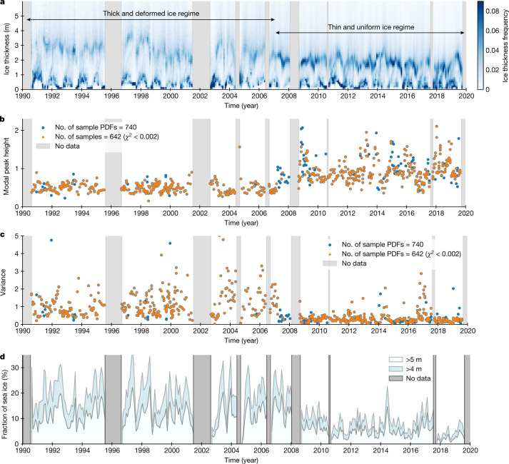
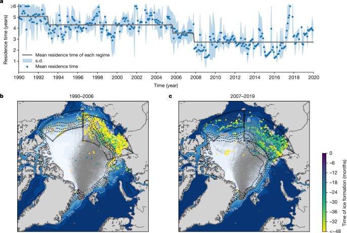
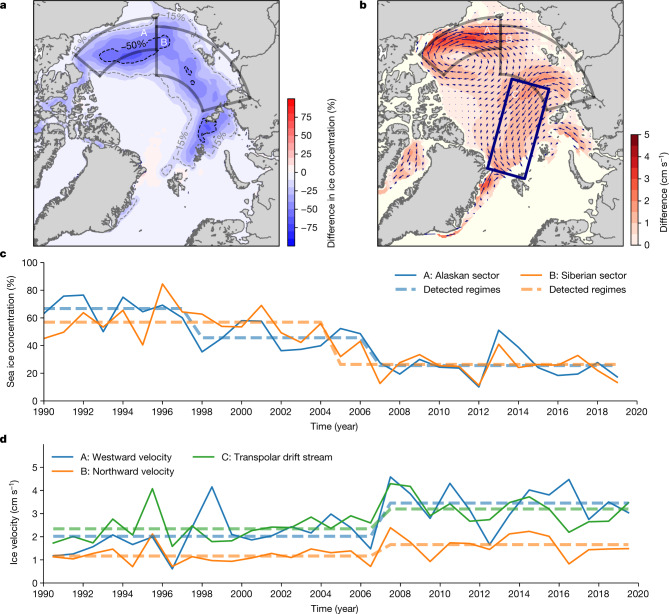
Manifestations of climate change are often shown as gradual changes in physical or biogeochemical properties¹. Components of the climate system, however, can show stepwise shifts from one regime to another, as a nonlinear response of the system to a changing forcing². Here we show that the Arctic sea ice regime shifted in 2007 from thicker and deformed to thinner and more uniform ice cover. Continuous sea ice monitoring in the Fram Strait over the last three decades revealed the shift. After the shift, the fraction of thick and deformed ice dropped by half and has not recovered to date. The timing of the shift was preceded by a two-step reduction in residence time of sea ice in the Arctic Basin, initiated first in 2005 and followed by 2007. We demonstrate that a simple model describing the stochastic process of dynamic sea ice thickening explains the observed ice thickness changes as a result of the reduced residence time. Our study highlights the long-lasting impact of climate change on the Arctic sea ice through reduced residence time and its connection to the coupled ocean-sea ice processes in the adjacent marginal seas and shelves of the Arctic Ocean.

Fig. 1. Map of Arctic Ocean and sea ice thickness distribution in the Fram Strait.

a, Arctic Ocean and its marginal seas, with winter sea ice concentration (1980–2018 mean, white-blue shading, calculated from OSI SAF), ice drift field (blue arrows, Polar Pathfinder Daily 25 km EASE-Grid Sea Ice Motion Vectors v.4.1), 83 ice-tethered buoy tracks that arrived in the Fram Strait (green lines) and TPD Stream (yellow shade). The buoy tracks were obtained from the International Arctic Buoy Programme. The Fram Strait Arctic Outflow Observatory is shown by the red bar. b, Mean sea ice thickness distribution in the Fram Strait before and after 2007. The distributions were derived on a monthly basis by all available ULS data from 1990 to 2019 (described in the Methods) and averaged across two periods: 1990–2006 and 2007–2019. The Matplotlib basemap toolkit was used to plot the map.

Fig. 2. Sea ice thickness properties observed in the Fram Strait in the last three decades.

a–d, Time series of sea ice thickness distribution (a), modal peak height (b) and variance of ice thickness distributions (c), and fraction of sea ice thicker than two thresholds, that is, 4 m and 5 m, respectively (d). In b,c, χ² is a sum of the squared residuals at each log-normal function fitting. Derivations of the ice thickness distribution, modal peak height and variance are described in the Methods.

Fig. 3. Residence time and origins of sea ice in the Arctic Ocean that reached the Fram Strait.

a–c, Time series of residence time of ice floes in the Arctic Basin (a) and origins and pathways of ice floes before (b) and after 2007 (c). a, The abscissa references the time of arrival in the Fram Strait. The grey line shows the mean residence time in each regime detected by sequential t-test analysis of regime shifts. b,c, The location of the dots depicts areas of sea ice formation, while the colour of the dots indicates the time of sea ice formation relative to their arrival in the Fram Strait. The grey clouds in b and c show the trajectories of ice floes from their origins to the Fram Strait. The background colour (navy–white shading) in b and c shows the mean sea ice concentration in September for the corresponding periods (OSI SAF). The contours of the mean sea ice concentration are represented by the dashed lines (80%, 70%, 60% and 50% contours shown in black and 15% contour shown in white). Two polygons indicate the sea ice formation area in the Alaskan (A) and Siberian (B) sectors: the time series of sea ice concentration and ice drift speed in these areas are shown in Fig. 4. See the Methods for details of the backward trajectory calculation and residence time estimates. The Matplotlib basemap toolkit was used to plot the map.

Fig. 4. Changes of sea ice concentration and sea ice motion.

a,b, Difference of September sea ice concentration (a) and ice drift speed (b) between the two periods: 1990–2006 and 2007–2019. c,d, Time series of mean sea ice concentration in September (c) and mean sea ice drift speed in selected regions (d). a, The positive (negative) values indicate increase (decrease) in the latter period. b, The difference in sea ice drift vector is shown by the arrows, while its magnitude is shown by the colour. The difference in sea ice drift field in b was calculated from ice drift vectors from December to May. The time series in c are the areal average of the Alaskan (A) and Siberian sectors (B) shown by the solid black polygon in a, while those in d are the areal average of A, B and C: the TPD Stream is shown by the rectangular box labelled C. The ice drift speed of the TPD in d shows the annual mean ice drift speed in box C (vector component parallel to the main axis of box C, positive value oriented to the Fram Strait), whereas those in A and B are calculated without three summer months (August to October) to exclude under-represented ice motion due to very low spatial coverage in recent years. c,d, The dashed lines indicate the detected regimes (Extended Data Table 1). Sea ice concentration from OSI SAF and sea ice drift from Polar Pathfinder Daily 25 km EASE-Grid Sea Ice Motion Vectors v.4.1 (ref. ) were used to derive the variables. The Matplotlib basemap toolkit was used to plot the map.

Fig. 5. Ice thickness distributions obtained from the stochastic model of dynamic ice thickening.

Probability density functions of X_m for different values of m. The smaller m corresponds to a shorter residence time of sea ice in the Arctic Ocean. See the Methods for the descriptions.

Extended Data Fig. 1. Difference of sea surface temperature (SST) between two periods 1990–2006 and 2007–2019.

(a) Difference of mean September SST estimated from Daily Optimum Interpolated Sea Surface Temperature data set (DOISST ver. 2.1), (b) Time series of mean September SST in sea ice formation areas A and B, calculated from DOISST. (c) Difference of upper ocean temperature (July to September mean, 0–20 m) between the two periods calculated from in-situ observational datasets^,. The dashed lines in (b) denote detected regimes by sequential t-test described in Methods. Matplotlib basemap toolkit is used to plot the map.

Extended Data Fig. 2. Mean residence time of sea ice in the Siberian sector and the central Arctic.

The residence time is calculated by the backward trajectories described in Methods. The central Arctic is defined being outside of the two polygons A and B. The ice formation areas A and B are shown in Fig. 3b in the main text. The solid lines denote regimes detected by the sequential t-test described in Methods.

Extended Data Fig. 3. Time series of ice thickness distribution in Fram Strait including open water fraction.

The thickness distributions are derived including open water fraction (i.e., zero thickness bin) on monthly basis. Data processing procedures are described in Methods.

Extended Data Fig. 4. Time series of ice thickness distribution in each site.

Time series of ice thickness distribution observed by each moored ULS (F11 to F14) in Fram Strait. The distributions are derived on monthly basis. Data processing procedures are described in Methods.

Extended Data Fig. 5. Examples of winter and summer sea ice thickness distributions in Fram Strait.

Examples of sea ice thickness distributions and corresponding fitted lognormal functions in March (top three rows) and September (bottom three rows). The blue, orange and green lines show ice thickness distribution, fitted lognormal function, and cut-off threshold, respectively. The plots are shown for every three years if data are available. Data processing procedures are described in Methods.

Extended Data Fig. 6. Time series of modal peak height and fitting parameters.

Time series of (a) modal thickness, (b) modal peak height, (c) variance, and (d, e) fitting parameters of lognormal functions. Data processing procedures are described in Methods. The gray solid lines in panels (a–c) show regimes detected by the sequential t-test.

Extended Data Fig. 7. Change of sea level pressure and wind pattern after the regime shift.

Difference of sea level pressure (SLP) and wind field between two periods 1990–2006 and 2007–2019, in (a) summer (from June to November) and (b) winter (from December to May), and (c) time series of annual mean 10 m wind averaged in the three polygons shown in panels (a) and (b). The polygons show (a) Alaskan sector, (b) Siberian sector, and (c) the area representing the Transpolar Drift Stream. The mean speed in the rectangular box C is the component of 10 m wind vector parallel to the major axis of the box (positive wind speed orients to the Fram Strait). SLP and 10 m wind data are taken from ERA5. Matplotlib basemap toolkit is used to plot the map.

Extended Data Fig. 8. Fraction of thick sea ice with detected regimes.

Fraction of thick sea ice (> 5 m and > 4m) observed in Fram Strait. Data processing procedures are described in Methods. The solid and dashed lines denote regimes detected by the sequential t-test.

References

1. Fox-Kemper, B. et al. Ocean, cryosphere and sea level change. IPCC Climate Change 2021: The Physical Science Basis (eds Masson-Delmotte, V. et al.) (Cambridge Univ. Press, 2021).
1. Cooper GS, Willcock S, Dearing JA. Regime shifts occur disproportionately faster in larger ecosystems. Nat. Commun. 2020;11:1175. doi: 10.1038/s41467-020-15029-x. - DOI - PMC - PubMed
1. Druckenmiller, M. L., Moon, T. & Thoman, R. (eds) State of the Climate in 2020: The Arctic. Bull. Am. Meteorol. Soc. 102, S263–S315 (American Meteorological Society, 2020).
1. Frey KE, Moore GWK, Cooper LW, Grebmeier JM. Divergent patterns of recent sea ice cover across the Bering, Chukchi, and Beaufort Seas of the Pacific Arctic Region. Prog. Oceanogr. 2015;136:32–49. doi: 10.1016/j.pocean.2015.05.009. - DOI
1. Serreze MC, Holland MM, Stroeve J. Perspectives on the Arctic’s shrinking sea-ice cover. Science. 2007;315:1533–1536. doi: 10.1126/science.1139426. - DOI - PubMed
Publication types