Partner choice, confounding and trait convergence all contribute to phenotypic partner similarity

Abstract

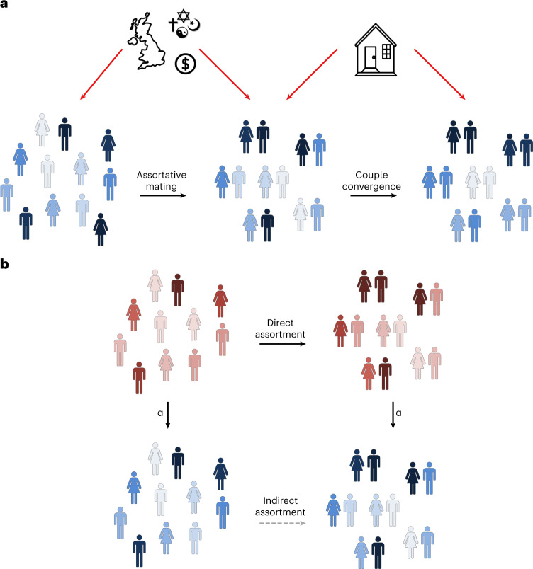
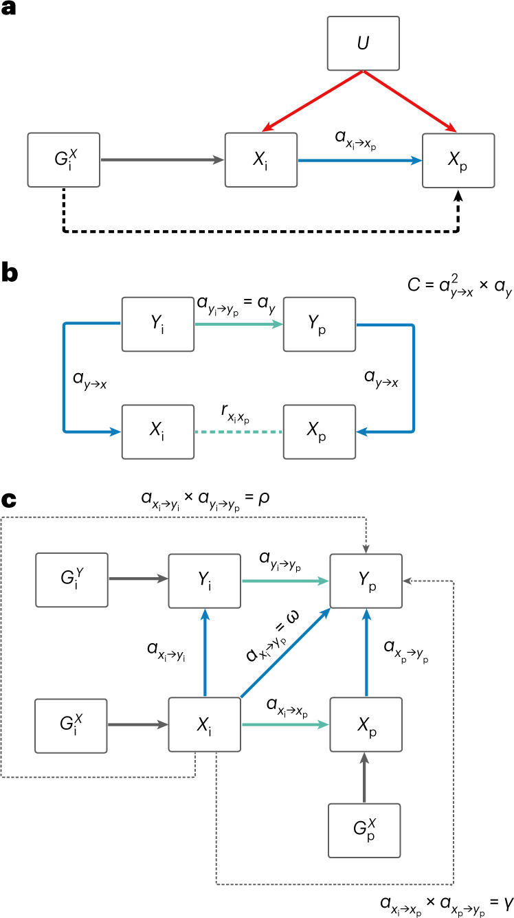
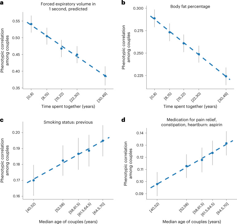
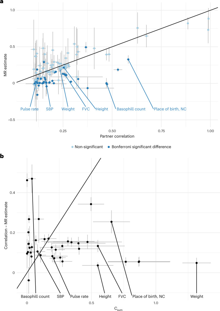
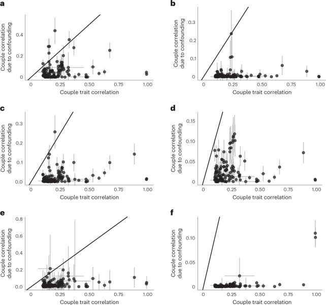
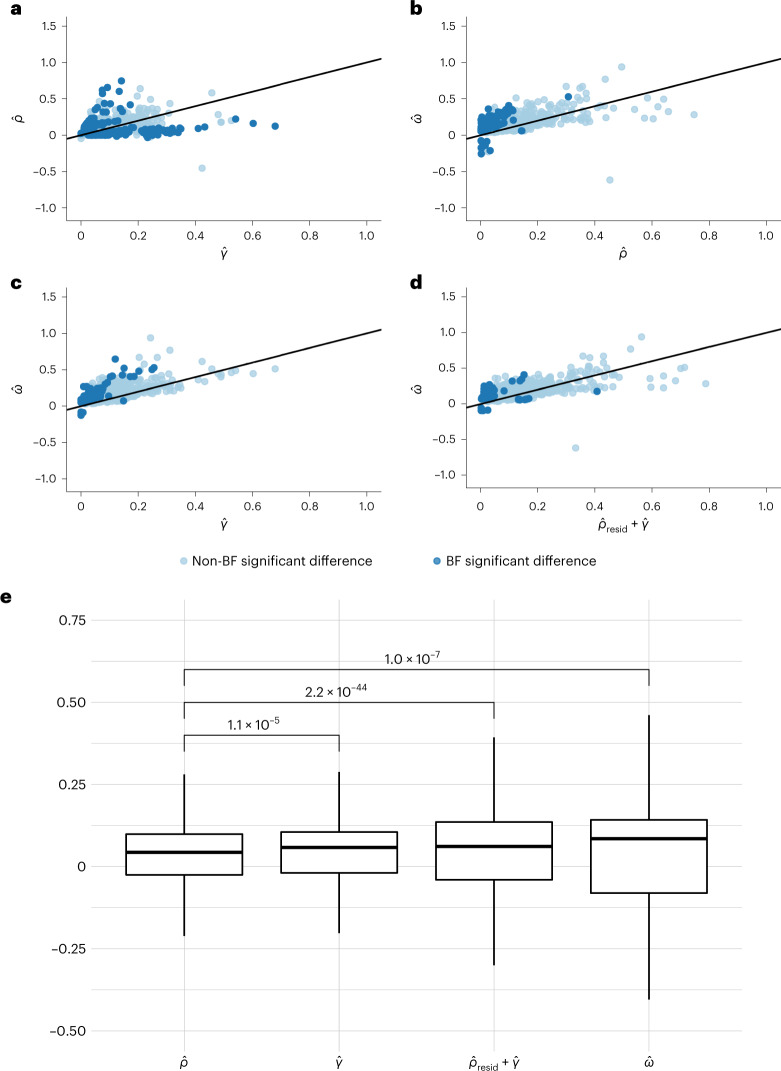
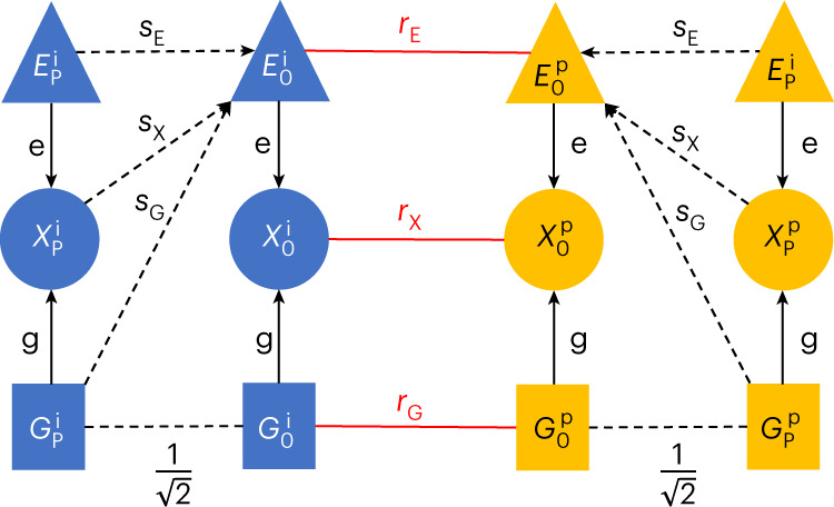
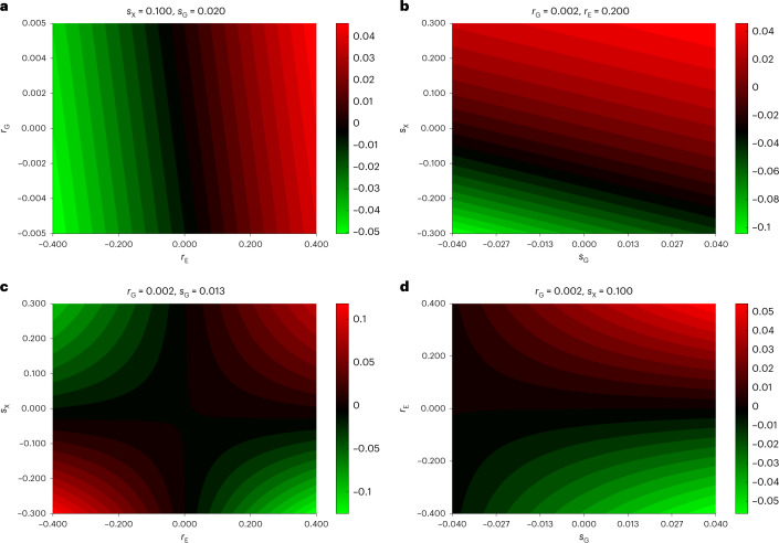
Partners are often similar in terms of their physical and behavioural traits, such as their education, political affiliation and height. However, it is currently unclear what exactly causes this similarity-partner choice, partner influence increasing similarity over time or confounding factors such as shared environment or indirect assortment. Here, we applied Mendelian randomization to the data of 51,664 couples in the UK Biobank and investigated partner similarity in 118 traits. We found evidence of partner choice for 64 traits, 40 of which had larger phenotypic correlation than causal effect. This suggests that confounders contribute to trait similarity, among which household income, overall health rating and education accounted for 29.8, 14.1 and 11.6% of correlations between partners, respectively. Finally, mediation analysis revealed that most causal associations between different traits in the two partners are indirect. In summary, our results show the mechanisms through which indirect assortment increases the observed partner similarity.

Fig. 1. Partner similarity framework.

a, Illustrates a trait (given by the colour blue) which shows increased similarity between partners, either directly (through mate choice) or due to confounding factors such as shared geography, cultural or religious status or socioeconomic measures. Subsequently, this trait may also undergo postmating convergence, which could be due to direct causal influence from one partner on the other (that is, through imitation or influence) or due to confounding factors such as shared environment. b, Illustrates a trait which shows increased similarity among couples (given by the blue trait); however, this assortment is only observed because of a causal effect (α) that exists between another trait (shown in red) acting on the blue trait. For example, if direct assortment occurs under a trait such as BMI (that is, couples intentionally select partners of similar BMI as themselves), phenotypic correlation will also be observed at all traits which have a causal effect on BMI, such as blood pressure, fasting glucose and so on.

Fig. 2. MR schematic within couples.

a, Illustrates the causal effect among couples with a single trait $\left({\alpha }_{x_{\mathrm{i}}\to x_{\mathrm{p}}}\right)$, where G represents genetic variant(s), X represents a single trait (in an index individual (X_i) and a partner (X_p)) and U represents confounding factors that are not associated with genetic variance owing to the random distribution of alleles at conception. Throughout the paper subscript i and p refer to the index and the partner, respectively. b, Directed acyclic graph illustrates the impact a confounder (trait Y) could have on the phenotypic correlation between partners for a given trait X ($r_{x_{\mathrm{i}}{x}_{\mathrm{p}}}$). Correlation due to confounding can be calculated as $C={\alpha }_{y\to x}^2\times {\alpha }_y$. c, Represents the expanded causal network involving two traits and the various estimated causal paths from trait X of an index case ($X_{\mathrm{i}}$) to a phenotype Y in the partner ($Y_{\mathrm{p}}$) given by ω, γ and ρ. Cross-trait causal effects from $X_{\mathrm{i}}$ to $Y_{\mathrm{p}}$ (ω) can be summarized by three possible (non-independent) scenarios: (1) $X_{\mathrm{i}}$ could exert a causal effect on $X_{\mathrm{p}}$, followed by $X_{\mathrm{p}}$ having a causal effect on $Y_{\mathrm{p}}$ in the partner alone (γ); (2) the reverse could occur whereby $X_{\mathrm{i}}$ has a causal effect on $Y_{\mathrm{i}}$ in the index alone, followed by a causal effect of $Y_{\mathrm{i}}$ case on $Y_{\mathrm{p}}$ (ρ); or (3) there could be other mechanisms, either acting directly or through other unmeasured or unconsidered variables. To quantify ρ, we first estimated the causal effect of $Y_{\mathrm{i}}$ on $Y_{\mathrm{p}}$ in MVMR (not illustrated) to exclude any residual effect of X on phenotype Y from index to partner. These three scenarios could also act in some combination. Therefore, the ω estimate would capture the paths of γ, ρ and other mechanisms combined. In both a and c, cross-partner causal effects are given by blue arrows and same-person causal effects are given by green arrows.

Fig. 3. Phenotypic correlation for selected traits by time spent together and age of couples.

a–d, Scatterplots show the phenotypic correlation for four selected traits among couples within different bins. Couples were binned by time spent together (proxied by the time lived at the same household) (a,b) and median age (c,d). The four panels show correlations for four different traits: forced expiratory volume (a), body fat percentage (b), previous smoker (c) and aspirin use (d).

Fig. 4. Phenotypic correlation in couples versus causal effects and evidence of confounder traits impacting the discrepant estimates.

a, Scatterplot shows the within-couple standardized MR estimates (${\alpha }_{x_{\mathrm{i}}\to x_{\mathrm{p}}}$) versus the phenotypic correlation among couples $\left(r_{x_{\mathrm{i}}{x}_{\mathrm{p}}}\right)$. The centre of the confidence interval (CI) is the estimate for the corresponding parameter and error bars represent 95% CIs. A two-tailed Z test was used to test for a significant difference between the estimates. After adjusting for the number of effective tests (P < 0.05/66), 43 significant differences were identified (shown in dark blue), where 3 traits showed larger MR estimates compared to correlation and 40 traits showed larger correlation compared to MR estimates. The identity line is shown in black. Labelled pairs are discussed in the main text. b, Scatterplot shows the difference in phenotypic correlation and MR estimate versus the C_sum value (estimating the correlation induced by measured (uncorrelated) confounders) for each trait where the phenotypic correlation was greater than the MR estimate (number of traits = 39); error bars represent 95% CIs. The identity line is shown in black. FVC, forced vital capacity; NC, north coordinate; SBP, systolic blood pressure.

Fig. 5. Global confounding impact of select traits on couple phenotypic correlation.

a–f, Scatterplots of couple correlation due to confounding versus the phenotypic trait correlation among couples for selected potential confounder traits (Z). The couple correlation due to confounding for each trait X was calculated for each confounder Y as $C={\alpha }_{y\to x}^2\times {\alpha }_{y_{\mathrm{i}}\to y_{\mathrm{p}}}$. In the case of birthplace coordinates, C values were summed across the two (independent) north and east coordinates. The centre of the CI is the estimator value and the error bars represent the 95% CI. These confidence intervals for the correlations shown on the x axis are based on the number of couples shown in the ‘n_pairs’ column of Supplementary Table 2. The CI for confounder-induced correlation was computed as 1.96 times the s.e. of the estimator ${\widehat{\alpha }}_{y\to x}^2\times {\widehat{\alpha }}_{y_{\mathrm{i}}\to y_{\mathrm{p}}}$, the computation of which is described in the Methods. For each trait in the pipeline, we tested how the contribution of six confounder traits (average total household income before tax (a), current tobacco smoking (b), age completed full-time education (c), overall health rating (d), sports club or gym user (e) and place of birth coordinates (f)) could impact the phenotypic couple correlation. The identity line is shown in black.

Fig. 6. Comparison of causal paths between two traits within couples.

a–d, We estimated various causal effect paths (ρ, γ and ω, see Fig. 2c) from a phenotype of the index case ($X_{\mathrm{i}}$) to another phenotype of its partner ($Y_{\mathrm{p}}$) for the 1,088 trait pairs with significant MR effects among couples ($p_{\widehat{\omega }}$ < 0.05/[66²]) and trait pair correlation <0.8. Panel (a) provides a scatter plot for 𝜌̂ against 𝛾̂ ; panel (b) for 𝜔̂ against 𝜌̂; panel (c) for 𝜔̂ against 𝛾̂ and panel (d) for 𝜔̂ against $\widehat{{\rho }_{\mathrm{resid}}}+\widehat{\gamma }$. The solid black line represents the linear regression fit. Dark blue dots indicate trait pairs with significant (after Bonferroni, BF, correction) difference between the respective parameters shown in the scatter plot, while light blue one mark the remaining traits. To calculate $\widehat{{\rho }_{\mathrm{r}\mathrm{e}\mathrm{s}\mathrm{i}\mathrm{d}}}+\hat{\gamma }$, we residualized $\widehat{\rho }$ for the effects of $\widehat{\gamma }$ ($\widehat{{\rho }_{\mathrm{resid}}}$) to ensure complete independence between the estimates and then added $\widehat{{\rho }_{\mathrm{resid}}}$ to $\widehat{\gamma }$ ($\widehat{{\rho }_{\mathrm{resid}}}+\widehat{\gamma }$). e, A box plot comparing the coefficients of the estimates among the trait pairs after removing 19 trait pairs where the sign did not match between any combination of the four coefficients. In the box plots, the lower and upper hinges correspond to the first and third quartiles and the middle bar corresponds to the median; the upper whisker is the largest point smaller than 1.5 times the interquartile range above the third quartile; the lower whisker is defined analogously. We used a two-sided paired t test to compare the presented estimates ($\widehat{\rho },\widehat{\gamma },\widehat{{\rho }_{\mathrm{resid}}}+\widehat{\gamma }$ and $\widehat{\omega }$).

Fig. 7. Modelling the impact of parental effect and AM on cross-sample MR.

The diagram represents the underlying joint model of parental effects and assortment. A focal trait (X) has genetic (G) and envionmental (E) components, with effect size g and e, respectively. Their subscripts can be O, F or M, referring to the offspring, the father or the mother, respectively. The superscripts can be either i or p, indicating the index individual or its partner. We allowed parental genetics, parental environment and the parental trait each to influence the offspring’s environment, with corresponding direct effect strengths s_G, s_E and s_X, respectively. Finally, couples are formed under direct assortments acting on G, E and X, leading to correlations r_G, r_E and r_X, respectively.

Fig. 8. The impact of various model parameters on MR bias.

We plotted the bias of the cross-sample MR estimates as a function of the proposed model parameters. Parameter $r_{\mathrm{G}}$ refers to direct genetic assortment, $r_{\mathrm{E}}$ to direct environmental assortment, $s_{\mathrm{G}}$ to direct parental genetic effect and $s_{\mathrm{X}}$ to direct parental trait effect. The different panels show the extent of bias when different pairs of parameters were covaried: $r_{\mathrm{G}},r_{\mathrm{E}}$ (a), $s_{\mathrm{G}},s_{\mathrm{X}}$ (b), $r_{\mathrm{E}},s_{\mathrm{X}}$ (c) and $s_{\mathrm{G}},r_{\mathrm{E}}$ (d).

References

1. Willoughby EA, et al. Parent contributions to the development of political attitudes in adoptive and biological families. Psychol. Sci. 2021;32:2023–2034. doi: 10.1177/09567976211021844. - DOI - PMC - PubMed
1. Kandler C, Bleidorn W, Riemann R. Left or right? Sources of political orientation: the roles of genetic factors, cultural transmission, assortative mating, and personality. J. Pers. Soc. Psychol. 2012;102:633–645. doi: 10.1037/a0025560. - DOI - PubMed
1. Silventoinen K, Kaprio J, Lahelma E, Viken RJ, Rose RJ. Assortative mating by body height and BMI: Finnish twins and their spouses. Am. J. Hum. Biol. 2003;15:620–627. doi: 10.1002/ajhb.10183. - DOI - PubMed
1. Maes HH, Neale MC, Eaves LJ. Genetic and environmental factors in relative body weight and human adiposity. Behav. Genet. 1997;27:325–351. doi: 10.1023/A:1025635913927. - DOI - PubMed
1. Keller MC. The genetic correlation between height and IQ: shared genes or assortative mating? PLoS Genet. 2013;9:e1003451. doi: 10.1371/journal.pgen.1003451. - DOI - PMC - PubMed
Publication types