Integrative modelling of reported case numbers and seroprevalence reveals time-dependent test efficiency and infectious contacts

Abstract

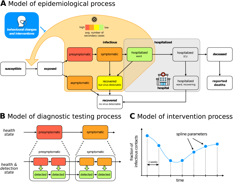
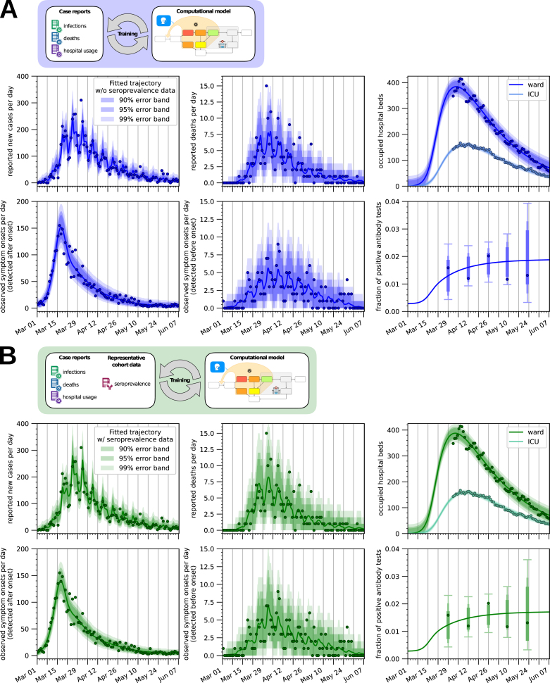
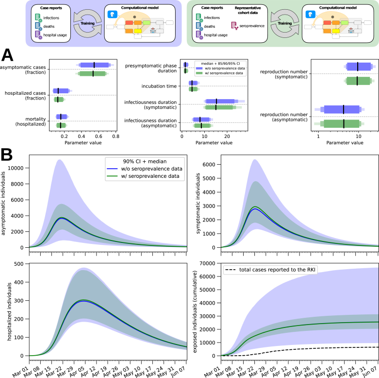
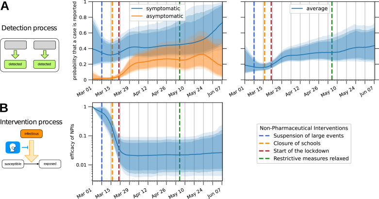
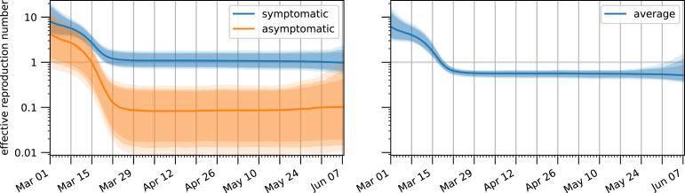
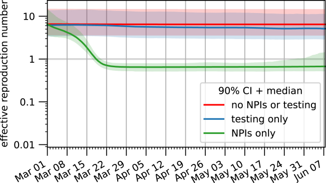
Mathematical models have been widely used during the ongoing SARS-CoV-2 pandemic for data interpretation, forecasting, and policy making. However, most models are based on officially reported case numbers, which depend on test availability and test strategies. The time dependence of these factors renders interpretation difficult and might even result in estimation biases. Here, we present a computational modelling framework that allows for the integration of reported case numbers with seroprevalence estimates obtained from representative population cohorts. To account for the time dependence of infection and testing rates, we embed flexible splines in an epidemiological model. The parameters of these splines are estimated, along with the other parameters, from the available data using a Bayesian approach. The application of this approach to the official case numbers reported for Munich (Germany) and the seroprevalence reported by the prospective COVID-19 Cohort Munich (KoCo19) provides first estimates for the time dependence of the under-reporting factor. Furthermore, we estimate how the effectiveness of non-pharmaceutical interventions and of the testing strategy evolves over time. Overall, our results show that the integration of temporally highly resolved and representative data is beneficial for accurate epidemiological analyses.

Keywords: COVID-19; Compartmental model; Parameter estimation; Uncertainty quantification.

Fig. 1

Structure of the compartment model. (A) High-level structure indicating possible transitions between various illness phases and hospitalization compartments. The delay between death and its reporting to the healthcare authorities is added in order to account for the lower number of deaths observed during weekends. Infectious phases are coloured with different colours encoding our a priori beliefs on the average number of secondary cases generated in a day by an individual in the corresponding compartment. We remark that such a number depends on the degree of infectiousness as well as the total number of inter-personal contacts. For example, on the one hand symptomatic individuals are more infectious than asymptomatic ones, but on the other they are much less likely to encounter other people due to their health condition. It is thus difficult to determine a priori which phase generates more secondary cases and as a first guess they are assigned the same colour in the figure. (B) Detailed structure of the compartment model. Each compartment is split into several sub-states in order to have Erlang-distributed transition times between compartments, and to explicitly model the testing process by tracking individuals reported to the health care authorities on a parallel but separate branch. (C) Time-dependent parameters (here the viral transmission reduction due to NPIs is used as an example) are modelled by splines which can be encoded inside the parameter vector by their values at the grid points.

Fig. 2

Model fit for Munich, Germany. Model simulation for the sampled parameter vector with the highest posterior probability compared with the observed data. In (A) only the case numbers reported by the Robert-Koch Institute and hospital usage for Munich are used for fitting, while in (B) seroprevalence data is also employed. The error bands show the range of plausible values for the observation, confirming that the noise models used are appropriate. In the bottom-right panels of (A, B), where the seroprevalence predicted by the model is plotted, the error bars are only shown at the observation times since the variance of each observation is linked to the number of total antibody tests carried out in each sub-batch.

Fig. 3

Uncertainty quantification. (A) 85%/90%/95% credible intervals (bars) and median value (line) for a subset of the model parameters. By reproduction number we mean the basic reproduction number in absence of NPIs and diagnostic testing (see Materials & Methods for more details on its computation). (B) The number of individuals in different compartments is plotted as a function of time for both the model fitted with seroprevalence data and the one fitted without. In the bottom-right panel the cumulative number of cases detected by the healthcare authorities is also plotted for reference. The bands correspond to 90% posterior credible intervals, while the solid line denotes the median value. (For interpretation of the references to colour in this figure legend, the reader is referred to the web version of this article.)

Fig. 4

Estimation of time-dependent parameters. The bands correspond to 85%/90%/95% posterior credible intervals, while the solid line denotes the median value. Dashed lines indicate at which dates specific NPIs were enforced/lifted. (A) Probability that an infected individual is detected and reported to the healthcare authorities before the virus is cleared from their system. The left plot shows such probabilities for symptomatic and asymptomatic infected individuals separately, while the right plot shows their weighted average, i.e. the probability that a generic infected individual is eventually detected. (B) Relative reduction in the number of infectious contacts due to NPIs and behavioural changes.

Fig. 5

Temporal evolution of the effective reproduction number. The left plot shows the effective reproduction numbers for symptomatic and asymptomatic infected individuals, while the right plot shows their weighted average, i.e. the reproduction number for a generic infected individual. The bands correspond to 85%/90%/95% posterior credible intervals, while the solid line denotes the median value.

Fig. 6

Relative importance of the detection process and the NPIs on the spread of the epidemic. Estimates for the reproduction number are plotted for three different scenarios: (red) neither diagnostic testing nor NPIs are employed; (blue) only diagnostic testing is performed; (green) only NPIs are applied. The bands correspond to the 90% posterior credible interval, while the solid line denotes the median value. (For interpretation of the references to colour in this figure legend, the reader is referred to the web version of this article.)

Fig. 7

Computation of the transit probabilities in a toy example. Let $p_i$ be the probability that an individual, starting in $X_1$, will transit through state $X_i$. We assume transitions between state $X_i$ and state $X_j$ occur at a rate $k_{ij}$ and that the possible transmissions are given in the graph shown in this figure. Then, $p_1=1$, $p_2=p_1$, $p_3=p_2{k}_{23}/(k_{23}+k_{26})$, $p_4=p_3{k}_{34}/(k_{34}+k_{35})$, $p_5=p_3-p_4$, $p_6=p_2-p_3$, $p_7=p_6$.

References

1. Barbarossa Maria Vittoria, Fuhrmann Jan, Meinke Jan H., Krieg Stefan, Varma Hridya Vinod, Castelletti Noemi, Lippert Thomas. Modeling the spread of COVID-19 in Germany: Early assessment and possible scenarios. PLOS ONE. 2020;15(9) doi: 10.1371/journal.pone.0238559. - DOI - PMC - PubMed
1. Beck E.M., Tolnay Stewart E. Analyzing historical count data. Hist. Methods. 1995;28(3):125–131. doi: 10.1080/01615440.1995.9956360. - DOI
1. Brauner Jan M., Mindermann Sören, Sharma Mrinank, Johnston David, Salvatier John, Gavenčiak Tomáš, Stephenson Anna B., Leech Gavin, Altman George, Mikulik Vladimir, Norman Alexander John, Monrad Joshua Teperowski, Besiroglu Tamay, Ge Hong, Hartwick Meghan A., Teh Yee Whye, Chindelevitch Leonid, Gal Yarin, Kulveit Jan. Inferring the effectiveness of government interventions against COVID-19. Science. 2021;371(6531) doi: 10.1126/science.abd9338. - DOI - PMC - PubMed
1. Catmull Edwin, Rom Raphael. In: Computer Aided Geometric Design. Barnhill Robert E., Riesenfeld Richard F., editors. Academic Press; 1974. A class of local interpolating splines; pp. 317–326. - DOI
1. Chan Stephen, Chu Jeffrey, Zhang Yuanyuan, Nadarajah Saralees. Count regression models for COVID-19. Physica A. 2021;563 doi: 10.1016/j.physa.2020.125460. - DOI - PMC - PubMed
Publication types