Multiomic signatures of body mass index identify heterogeneous health phenotypes and responses to a lifestyle intervention

Abstract

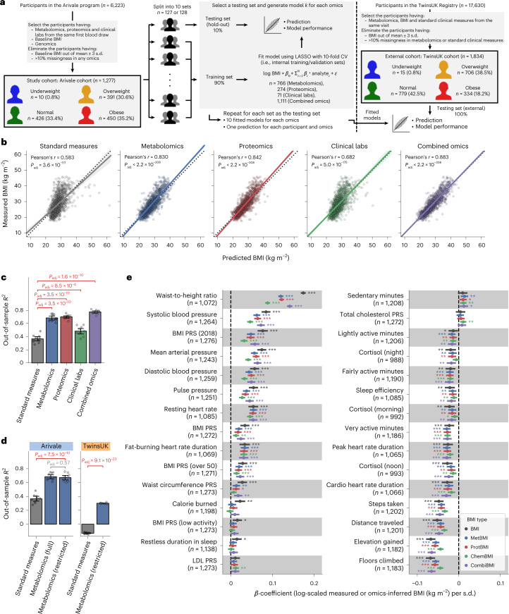
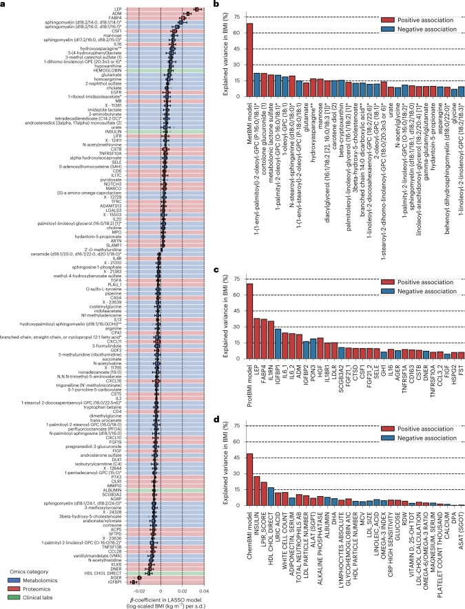
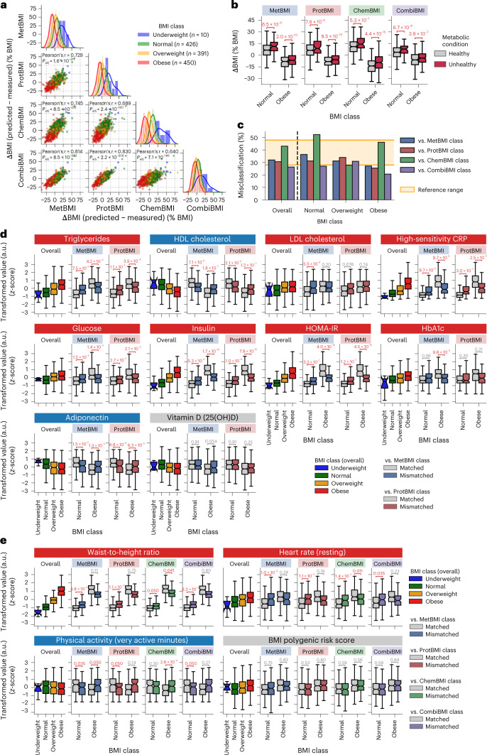
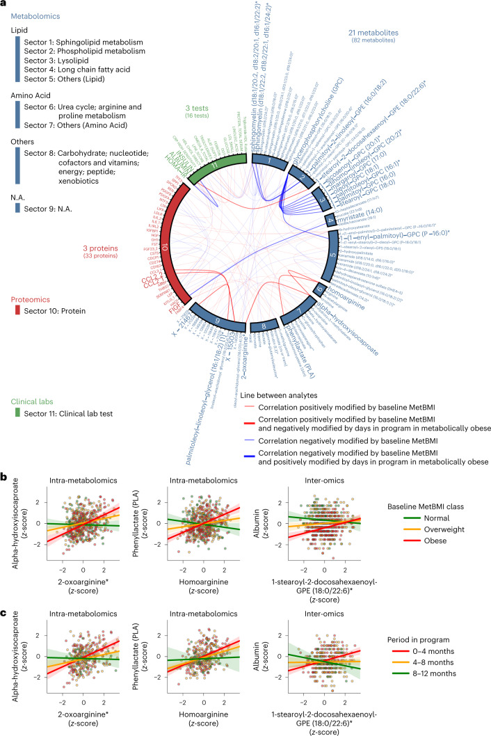
Multiomic profiling can reveal population heterogeneity for both health and disease states. Obesity drives a myriad of metabolic perturbations and is a risk factor for multiple chronic diseases. Here we report an atlas of cross-sectional and longitudinal changes in 1,111 blood analytes associated with variation in body mass index (BMI), as well as multiomic associations with host polygenic risk scores and gut microbiome composition, from a cohort of 1,277 individuals enrolled in a wellness program (Arivale). Machine learning model predictions of BMI from blood multiomics captured heterogeneous phenotypic states of host metabolism and gut microbiome composition better than BMI, which was also validated in an external cohort (TwinsUK). Moreover, longitudinal analyses identified variable BMI trajectories for different omics measures in response to a healthy lifestyle intervention; metabolomics-inferred BMI decreased to a greater extent than actual BMI, whereas proteomics-inferred BMI exhibited greater resistance to change. Our analyses further identified blood analyte-analyte associations that were modified by metabolomics-inferred BMI and partially reversed in individuals with metabolic obesity during the intervention. Taken together, our findings provide a blood atlas of the molecular perturbations associated with changes in obesity status, serving as a resource to quantify metabolic health for predictive and preventive medicine.

Fig. 1. Plasma multiomics captured 48–78% of the variance in BMI.

a, Overview of study cohorts and the omics-based BMI model generation. CV, cross-validation. b, Correlation between the measured and predicted BMIs. The solid line is the OLS linear regression line with 95% confidence interval, and the dotted line is measured BMI = predicted BMI. Standard measures: OLS linear regression model with sex, age, triglycerides, HDL cholesterol, LDL cholesterol, glucose, insulin and HOMA-IR as regressors; P_adj: adjusted P value of two-sided Pearson’s correlation test with the Benjamini–Hochberg method across the five categories (n = 1,277 participants). c,d, Model performance of each fitted BMI model. Out-of-sample R² was calculated from each corresponding hold-out testing set (Arivale: c,d) or from the external testing set (TwinsUK: d). Metabolomics (full): LASSO model trained by all 766 metabolites of the Arivale dataset; Metabolomics (restricted): LASSO model trained by the common 489 metabolites in the Arivale and TwinsUK datasets (Extended Data Fig. 3 and Methods); P_adj: adjusted P value of two-sided Welch’s t-test with the Benjamini–Hochberg method across the four (c) or three (d) comparisons. Data: mean with 95% confidence interval, n = 10 models. Note that Standard measures and Metabolomics (full) of Arivale in d are the same with corresponding ones in c. e, Association between omics-inferred BMI and physiological feature. For each of the 51 numeric physiological features (Supplementary Data 4), β-coefficient was estimated using OLS linear regression model with the measured or omics-inferred BMI as a dependent variable and sex, age and ancestry principal components as covariates. Presented are the 30 features that were significantly associated with at least one of the BMI types after multiple testing adjustment with the Benjamini–Hochberg method across the 255 (51 features × 5 BMI types) regressions. n, number of assessed participants. Data: estimate with 95% confidence interval. *Adjusted P < 0.05, **adjusted P < 0.01, ***adjusted P < 0.001. All exact values of test summaries are found in Supplementary Data 4 and 10.

Fig. 2. Omics-based BMI estimates captured the variance in BMI better than any single analyte.

a, The variables that were retained across all ten CombiBMI models (132 analytes: 77 metabolites, 51 proteins and four clinical laboratory tests). β-coefficient was obtained from the fitted CombiBMI model with LASSO linear regression (Supplementary Data 3). Each background color corresponds to the analyte category. Data: the standard box plot (Methods), n = 10 models. b–d, Univariate explained variance in BMI by each metabolite (b), protein (c) or clinical laboratory test (d). BMI was independently regressed on each of the analytes that were retained in at least one of the ten LASSO models (209 metabolites, 74 proteins and 41 clinical laboratory tests; Supplementary Data 5), using OLS linear regression with sex, age and ancestry principal components as covariates. Multiple testing was adjusted with the Benjamini–Hochberg method across the 210 (b), 75 (c) or 42 (d) regressions, including each omics-based BMI model as reference. Among the analytes that were significantly associated with BMI (180 metabolites, 63 proteins and 30 clinical laboratory tests), only the top 30 significant analytes are presented with their univariate variances. All exact values of test summaries are found in Supplementary Data 5.

Fig. 3. Metabolic heterogeneity was responsible for the high rate of misclassification within the standard BMI classes.

a, Difference of the omics-inferred BMI from the measured BMI (ΔBMI). P_adj: adjusted P value of two-sided Pearson’s correlation test with the Benjamini–Hochberg method across the six combinations (n, number of participants in each BMI class; total n = 1,277 participants). The line in the histogram panel indicates the kernel density estimate. b, Difference in ΔBMI between clinically defined metabolic health conditions within the normal or obese BMI class. Each comparison value indicates adjusted P value, calculated from OLS linear regression with BMI, sex, age and ancestry principal components as covariates while adjusting multiple testing with the Benjamini–Hochberg method across the eight (2 BMI classes × 4 omics categories) regressions. c, Misclassification rate of overall cohort or each BMI class against the omics-inferred BMI class. Reference range: the previously reported misclassification rate^,. The underweight BMI class is not presented owing to small sample size, but its misclassification rate was 80% against CombiBMI class and 100% against the others. d,e, Difference in the obesity-related clinical blood marker (d) or BMI-associated physiological feature (e) between the matched and mismatched groups within the normal or obese BMI class. Each comparison value indicates adjusted P value, calculated from OLS linear regression with BMI, sex, age and ancestry principal components as covariates while adjusting multiple testing with the Benjamini–Hochberg method across the 40 (d, 2 BMI classes × 2 omics categories × 10 markers) or 216 (e, 2 BMI classes × 4 omics categories × 27 features) regressions. Four of the 27 features that were significantly associated with BMI (Fig. 1c) are representatively presented in e, and the other results are found in Supplementary Data 6. 25(OH)D, 25-hydroxyvitamin D; a.u., arbitrary units. b,d,e, Data: the standard box plot (Methods); n = 373 (b, Healthy in Normal), 49 (b, Unhealthy in Normal), 208 (b, Healthy in Obese) or 241 (b, Unhealthy in Obese) participants (see Supplementary Data 6 for each sample size in d and e). All exact values of test summaries are found in Supplementary Data 6 and 10.

Fig. 4. Metabolomics-inferred BMI reflected gut microbiome profiles better than BMI.

a, Overview of study cohorts and the gut microbiome-based obesity classifier generation. CV, cross-validation; RF, random forest. b, Difference in gut microbiome α-diversity between the matched and mismatched groups within the normal or obese BMI class. Each comparison value indicates adjusted P value, calculated from OLS linear regression with BMI, sex, age and ancestry principal components as covariates while adjusting multiple testing with the Benjamini–Hochberg method across the 24 (2 BMI classes × 4 omics categories × 3 metrics) regressions. Data: the standard box plot (Methods); n = 240 (Normal) or 260 (Obese) participants (see Supplementary Data 6 for each sample size). a.u., arbitrary units. c,e, ROC curve of the gut microbiome-based model classifying participants to the normal versus obese class in the Arivale (c) or TwinsUK (e) cohort. Each ROC curve was generated from the overall participants: n = 500 (c, BMI class), 427 (c, MetBMI class), 209 (e, BMI class) or 145 (e, MetBMI class) participants. The dashed line indicates a random classification line. P: P value of two-sided unpaired DeLong’s test. d,f, Comparison of model performance between the BMI and MetBMI classifiers in the Arivale (d) or TwinsUK (f) cohort. Out-of-sample metric value was calculated from each corresponding hold-out testing set. Data: mean with 95% confidence interval, n = 5 models. P: P value of two-sided Welch’s t-test. All exact values of test summaries are found in Supplementary Data 6 and 10.

Fig. 5. Metabolic health of the metabolically obese group was improved during a healthy lifestyle intervention program.

a, Overview of the longitudinal analysis using omics-inferred BMI. b,c, Longitudinal change in the omics-inferred BMI within the overall cohort (b) or within each baseline BMI class (c). Average trajectory of each measured or omics-inferred BMI was independently estimated using LMM with random effects for each participant (Methods) in the overall cohort (b) or in each baseline BMI class-stratified group (c). d,e, Longitudinal change in MetBMI of the misclassified participants within the normal (d) or obese (e) BMI class. Average trajectory of each BMI or MetBMI was independently estimated using the above LMM with the baseline misclassification of BMI class against MetBMI class as additional fixed effects (Methods) in each baseline BMI class-stratified group. b–e, The dashed line corresponds to the baseline value of each estimate. Data: mean with 95% confidence interval; n = 608 (b), 222 (c, Normal), 185 (c, Overweight), 196 (c, Obese), 137 (d, Matched), 85 (d, Mismatched), 139 (e, Matched) or 57 (e, Mismatched) participants.

Fig. 6. Plasma analyte correlation network in the metabolically obese group shifted toward a structure observed in a metabolically healthier state during a healthy lifestyle intervention program.

a, Cross-omic interactions modified by MetBMI and days in the program. For each of the 608,856 pairwise relationships of plasma analytes (766 metabolites, 274 proteomics and 64 clinical laboratory tests), the baseline relationship between analyte–analyte pair and MetBMI within the Arivale subcohort (Fig. 5a; 608 participants) was assessed using their interaction term in each GLM (Methods) while adjusting multiple testing with the Benjamini–Hochberg method. The 100 analyte–analyte pairs (82 metabolites, 33 proteins and 16 clinical laboratory tests) that were significantly modified by the baseline MetBMI are presented. For each of these 100 pairs, the longitudinal relationship between analyte–analyte pair and days in the program within the metabolically obese group (that is, the baseline obese MetBMI class; 182 participants) was further assessed using their interaction term in each GEE (Methods) while adjusting multiple testing with the Benjamini–Hochberg method. The 27 analyte–analyte pairs (21 metabolites, three proteins and three clinical laboratory tests) that were significantly modified by days in the program are highlighted by line width and label font size. N.A., not available. All exact values of test summaries are found in Supplementary Data 7. b,c, Representative examples of the analyte–analyte pair that was significantly modified by both baseline MetBMI (b) and days in the program (c) in a. The solid line in each panel is the OLS linear regression line with 95% confidence interval. n = 530 (b, left), 553 (b, center) or 566 (b, right) participants; n = 324 (c, left), 339 (c, center) or 347 (c, right) measurements from the 182 participants of the metabolically obese group. Of note, data points outside of plot range are trimmed in these presentations.

Extended Data Fig. 1. Demographic information of study cohorts.

a–c, Demographic information of the Arivale study cohort (Fig. 1a, n = 1,277 participants). d–f, Demographic information of the TwinsUK study cohort (Fig. 1a, n = 1,834 participants). a,b,d,e, Distribution of the baseline BMI (a,d) or age (b,e). n, number of participants. The solid and dashed lines indicate the kernel density estimate and the mean of BMI (a, Female: 28.6 kg m⁻²; a, Male: 28.1 kg m⁻²; d, Female: 26.2 kg m⁻²; d, Male: 27.1 kg m⁻²) or age (b, Female: 47.6 years; b, Male: 44.7 years; e, Female: 61.4 years; e, Male: 62.0 years), respectively. c,f, Composition of self-reported race (c) or ethnicity (f). The number in parentheses indicates the number of participants. All summary values are found in Supplementary Data 1.

Extended Data Fig. 2. Quality check of the LASSO modeling.

a,b, Pairwise correlation of all plasma analytes (a; Metabolomics: 766 metabolites, Proteomics: 274 proteins, Clinical labs: 71 clinical laboratory tests, Combined omics: 1,111 analytes) or the analytes that were retained across all ten LASSO models (b; Metabolomics: 62 metabolites, Proteomics: 30 proteins, Clinical labs: 20 clinical laboratory tests, Combined omics: 132 analytes). Each violin is scaled to have same width between the omics categories and represents the kernel density distribution with the standard boxplot (Methods). c, Hierarchical clustering and heatmap for the pairwise correlations of the analytes that were retained across all ten CombiBMI models (132 analytes: 77 metabolites, 51 proteins and four clinical laboratory tests). Of note, both upper and lower triangular sides of the symmetric matrix are visualized. d, Model performance of each fitted BMI model with sex stratification. Out-of-sample R² was calculated from each corresponding hold-out testing set. Standard measures: OLS linear regression model with sex, age, triglycerides, HDL cholesterol, LDL cholesterol, glucose, insulin and HOMA-IR as regressors; P_adj: adjusted P value of two-sided Welch’s t-test with the Benjamini–Hochberg method across the eight (four comparisons × two sexes) comparisons. Data: mean with 95% confidence interval, n = 10 models. All exact values of test summaries are found in Supplementary Data 10. Note that the sample size for modeling was different between female and male (Female: 821 participants versus Male: 456 participants). e–h, Transition of out-of-sample R² in the LASSO-modeling iteration analysis (Methods) for metabolomics (e), proteomics (f), clinical labs (g) or combined omics (h). The iteration is highlighted with shading color when the removed analyte is the variable that was retained across all the original ten models. Data: mean with 95% confidence interval, n = 10 models.

Extended Data Fig. 3. The restricted MetBMI model predominantly maintained the characteristics of the original full model.

a–c, Comparison of the MetBMI model between the main analyses (Arivale cohort) and the validation analyses (TwinsUK cohort). Full version: LASSO model trained by all 766 metabolites in the Arivale dataset, Restricted version: LASSO model trained by the common 489 metabolites in the Arivale and TwinsUK datasets (Methods). a, The number of the variables that were robustly retained across all ten MetBMI models. The number in square brackets indicates the number of the robustly retained metabolites that were derived from the common 489 metabolites. b, Correlation of the mean of β-coefficients in the ten MetBMI models. Only the robustly retained metabolites in either full version (37 metabolites) or restricted version (74 metabolites) were analyzed. c, Correlation of the MetBMI prediction. b,c, The solid line is the OLS linear regression line with 95% confidence interval, and the dotted line in c is the value in full version = the value in restricted version. P: P value of two-sided Pearson’s correlation test. n = 76 metabolites (b) or 1,277 participants (c). d, Correlation between the measured and predicted BMIs. The solid line is the OLS linear regression line with 95% confidence interval, and the dotted line is measured BMI = predicted BMI. Standard measures: OLS linear regression model with sex, age, triglycerides, HDL cholesterol, LDL cholesterol, glucose, insulin and HOMA-IR as regressors; Metabolomics: the restricted version of MetBMI model, corresponding to Metabolomics (restricted) in Fig. 1d; P_adj: adjusted P value of two-sided Pearson’s correlation test with the Benjamini–Hochberg method across the four (two categories × two cohorts) tests. n = 1,277 (Arivale) or 1,834 (TwinsUK) participants. All exact values of test summaries are found in Supplementary Data 10.

Extended Data Fig. 4. Omics-based BMI models were similar between LASSO and the other methods.

a, Model performance of each fitted BMI model. P_adj: adjusted P value of two-sided Welch’s t-test with the Benjamini–Hochberg method across the 12 (3 methods × 4 categories) comparisons. Data: mean with 95% confidence interval, n = 10 models. b, Correlation of the predicted BMI between LASSO and the other methods. The solid line is the OLS linear regression line with 95% confidence interval, and the dotted line is LASSO = the other method. P_adj: adjusted P value of two-sided Pearson’s correlation test with the Benjamini–Hochberg method across the 12 (3 methods × 4 categories) combinations. n = 1,277 participants. c–f, Comparison of the omics-based BMI model between LASSO and elastic net. c–e, The number of the variables that were robustly retained across all ten models. f, Correlation of the mean of β-coefficients in the ten models. Only the robustly retained analytes in either LASSO models or elastic net models were analyzed. The solid line is the OLS linear regression line with 95% confidence interval. P_adj: adjusted P value of two-sided Pearson’s correlation test with the Benjamini–Hochberg method across the four categories. n = 62 metabolites, 30 proteins, 20 clinical laboratory tests or 134 analytes. a,b,f, All exact values of test summaries are found in Supplementary Data 10. g, The top 30 variables that had the highest absolute value for the mean of β-coefficients in the ten ridge CombiBMI models. β-coefficient was obtained from the fitted CombiBMI model with ridge linear regression. Data: the standard box plot (Methods), n = 10 models. h, The top 30 variables that had the highest mean of feature importance in the ten random forest CombiBMI models. Feature importance was calculated as the normalized total reduction of the mean squared error. Data: mean with 95% confidence interval, n = 10 models.

Extended Data Fig. 5. Variable diversity and contribution to the omics-based BMI model were different between omics categories.

a–c, The variables that were retained across all ten MetBMI (a), ProtBMI (b) or ChemBMI (c) models (a: 62 metabolites, b: 30 proteins, c: 20 clinical laboratory tests). β-coefficient was obtained from the fitted omics-based BMI model with LASSO linear regression (Supplementary Data 3). Data: the standard boxplot (Methods), n = 10 models.

Extended Data Fig. 6. The metabolic heterogeneity within the standard BMI classes was validated with the TwinsUK cohort.

a, Difference in ΔMetBMI (that is, difference of MetBMI from the measured BMI) between clinically-defined metabolic health conditions. Each comparison value indicates adjusted P value, calculated from OLS linear regression with BMI, sex and age as covariates, while adjusting multiple testing with the Benjamini–Hochberg method across the four (two BMI classes × two cohorts) regressions. For Arivale cohort, ancestry principal components were also included in the covariates. MetBMI in Arivale was derived from the restricted version of MetBMI model (Extended Data Fig. 3 and Methods). b, Misclassification rate of overall cohort or each BMI class against MetBMI class. Arivale (full): based on the full version of MetBMI model in Extended Data Fig. 3 (that is, the same with the corresponding ones in Fig. 3c), Arivale (restricted): based on the restricted version of MetBMI model in Extended Data Fig. 3, Reference range: the previously reported misclassification rate^,. The underweight BMI class is not presented owing to small sample size, but its misclassification rate was 100% in both cohorts. c, Difference in the obesity-related phenotypic measure between the matched and mismatched groups in the TwinsUK cohort. Each comparison value indicates adjusted P value, calculated from OLS linear regression with BMI, sex and age as covariates, while adjusting multiple testing with the Benjamini–Hochberg method across the 24 (2 BMI classes × 12 measures) regressions. Percent total fat: percentage of total fat in the whole body, Android-to-gynoid: ratio of fat in the android region to fat in the gynoid region, BP: blood pressure, a.u.: arbitrary units. a,c, Data: the standard boxplot (Methods). See Supplementary Data 6 for the number of participants in each group. All exact values of test summaries are found in Supplementary Data 6 and 10.

Extended Data Fig. 7. Omics-based WHtR models consistently supported the findings of omics-based BMI models.

a, Overview of study cohort and the omics-based WHtR model generation. CV,cross-validation. b, Distribution of the baseline WHtR. c, Correlation between the measured WHtR and BMI. d, Correlation between the measured and predicted WHtRs. e, Model performance of each fitted WHtR model. f–i, Transition of out-of-sample R² in the LASSO-modeling iteration analysis (Methods) for metabolomics (f), proteomics (g), clinical labs (h) or combined omics (i). The iteration is highlighted with shading color when the removed analyte is the variable that was retained across all the original ten models. j, The variables that were retained across all ten CombiWHtR models (37 analytes: 18 metabolites, 15 proteins and four clinical laboratory tests). β-coefficient was obtained from the fitted CombiWHtR model (Supplementary Data 8). k, Univariate explained variance in WHtR by each analyte. Among the analytes that were significantly associated with WHtR (212 analytes; Methods), only the top 30 significant analytes are presented with their univariate variances. l, Difference of the omics-inferred WHtR from the measured WHtR (ΔWHtR). m, Difference in ΔWHtR between clinically-defined metabolic health conditions. Each comparison value indicates adjusted P value, calculated from OLS linear regression with WHtR, sex, age and ancestry principal components as covariates, while adjusting multiple testing with the Benjamini–Hochberg method across the eight (two BMI classes × four omics categories) regressions. P_adj: adjusted P value of two-sided Pearson’s correlation test (c,d,l) or Welch’s t-test (e) with the Benjamini–Hochberg method across the two sexes (c), five categories (d), four comparisons (e) or six combinations (l). Data: mean with 95% confidence interval (e–i) or the standard boxplot (j,m), n = 10 models (e–i,j) (see Supplementary Data 10 for each number of participants in m). All exact values of test summaries are found in Supplementary Data 9 and 10.

Extended Data Fig. 8. Predominant commonality with minor specificity was observed between the omics-based BMI and WHtR models.

a–d, Comparison of the omics-based LASSO model between BMI and WHtR. a–c, The number of the variables that were robustly retained across all ten LASSO models. d, Correlation of the mean of β-coefficients in the ten LASSO models. Only the robustly retained analytes in either BMI models or WHtR models were analyzed. e, Correlation between ΔBMI (that is, difference of the omics-inferred BMI from the measured BMI) and ΔWHtR (that is, difference of the omics-inferred WHtR from the measured WHtR). Only the participants having both BMI and WHtR were analyzed. d,e, The solid line is the OLS linear regression line with 95% confidence interval. P_adj: adjusted P value of two-sided Pearson’s correlation test with the Benjamini–Hochberg method across the four categories. n = 92 metabolites (d, Metabolomics), 36 proteins (d, Proteomics), 26 clinical laboratory tests (d, Clinical labs), 146 analytes (d, Combined omics) or 1,078 participants (e). All exact values of test summaries are found in Supplementary Data 10.

References

1. NCD Risk Factor Collaboration (NCD RisC). Trends in adult body-mass index in 200 countries from 1975 to 2014: a pooled analysis of 1698 population-based measurement studies with 19·2 million participants. Lancet387, 1377–1396 (2016). - PMC - PubMed
1. NCD Risk Factor Collaboration (NCD RisC).Worldwide trends in body-mass index, underweight, overweight, and obesity from 1975 to 2016: a pooled analysis of 2416 population-based measurement studies in 128·9 million children, adolescents, and adults. Lancet390, 2627–2642 (2017). - PMC - PubMed
1. Kopelman PG. Obesity as a medical problem. Nature. 2000;404:635–643. doi: 10.1038/35007508. - DOI - PubMed
1. Haslam DW, James WPT. Obesity. Lancet. 2005;366:1197–1209. doi: 10.1016/S0140-6736(05)67483-1. - DOI - PubMed
1. Kahn SE, Hull RL, Utzschneider KM. Mechanisms linking obesity to insulin resistance and type 2 diabetes. Nature. 2006;444:840–846. doi: 10.1038/nature05482. - DOI - PubMed
Publication types