. 2023 Mar;615(7954):892-899.
doi: 10.1038/s41586-023-05813-2. Epub 2023 Mar 22.

Population dynamics of head-direction neurons during drift and reorientation

Affiliations

Population dynamics of head-direction neurons during drift and reorientation

Zaki Ajabi et al. Nature. 2023 Mar.

Erratum in

Abstract

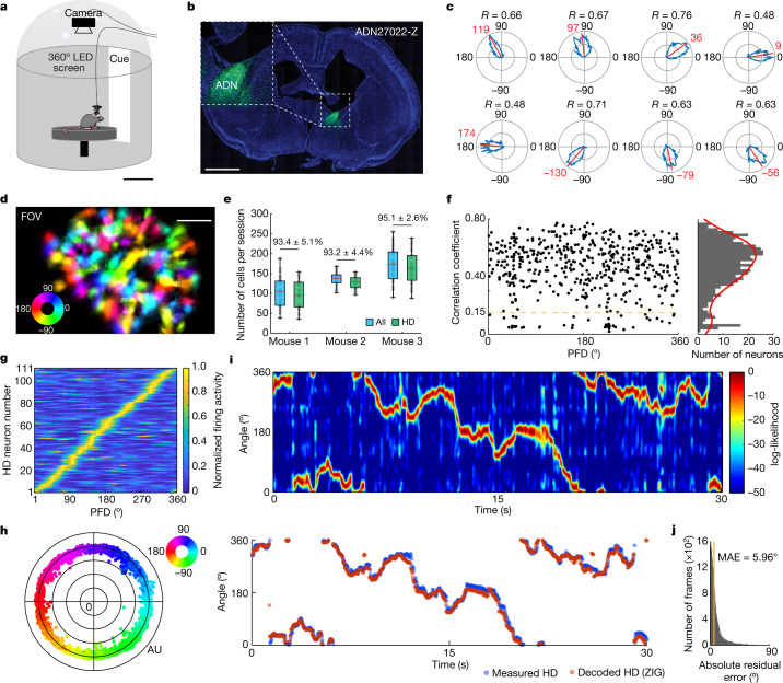
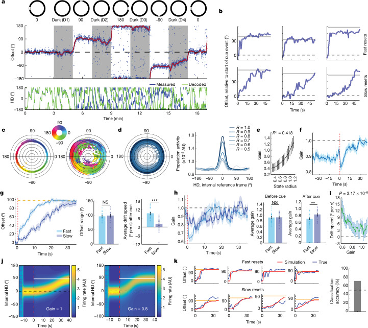
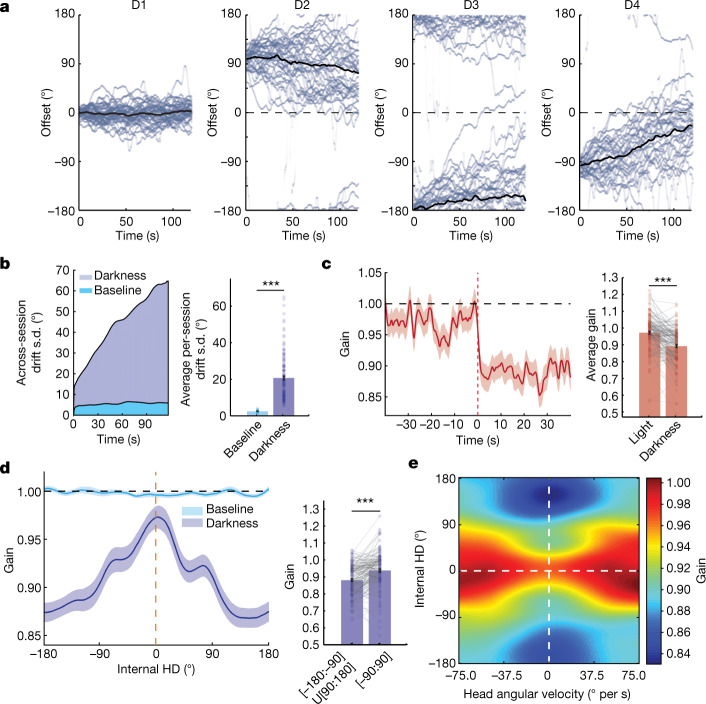
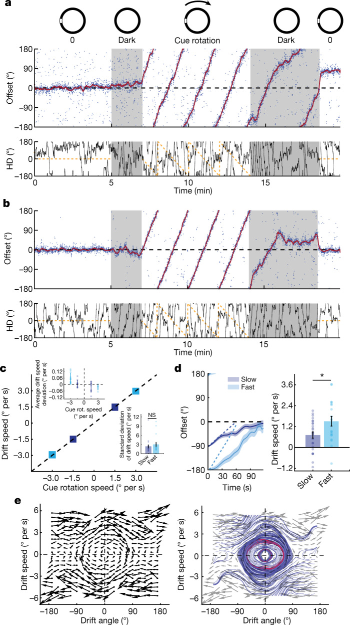
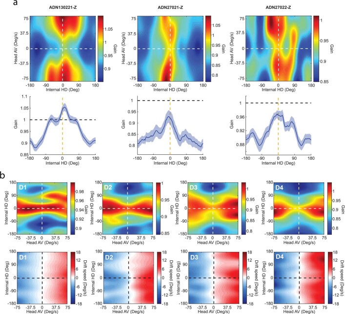
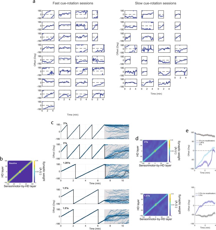
The head direction (HD) system functions as the brain's internal compass1,2, classically formalized as a one-dimensional ring attractor network3,4. In contrast to a globally consistent magnetic compass, the HD system does not have a universal reference frame. Instead, it anchors to local cues, maintaining a stable offset when cues rotate5-8 and drifting in the absence of referents5,8-10. However, questions about the mechanisms that underlie anchoring and drift remain unresolved and are best addressed at the population level. For example, the extent to which the one-dimensional description of population activity holds under conditions of reorientation and drift is unclear. Here we performed population recordings of thalamic HD cells using calcium imaging during controlled rotations of a visual landmark. Across experiments, population activity varied along a second dimension, which we refer to as network gain, especially under circumstances of cue conflict and ambiguity. Activity along this dimension predicted realignment and drift dynamics, including the speed of network realignment. In the dark, network gain maintained a 'memory trace' of the previously displayed landmark. Further experiments demonstrated that the HD network returned to its baseline orientation after brief, but not longer, exposures to a rotated cue. This experience dependence suggests that memory of previous associations between HD neurons and allocentric cues is maintained and influences the internal HD representation. Building on these results, we show that continuous rotation of a visual landmark induced rotation of the HD representation that persisted in darkness, demonstrating experience-dependent recalibration of the HD system. Finally, we propose a computational model to formalize how the neural compass flexibly adapts to changing environmental cues to maintain a reliable representation of HD. These results challenge classical one-dimensional interpretations of the HD system and provide insights into the interactions between this system and the cues to which it anchors.


Conflict of interest statement

The authors declare no competing interests.

Figures

Fig. 1
Fig. 1. Population recordings in the mouse ADN.
a, Schematic of the recording environment within a 360° LED screen. Scale bar, 20 cm. b, GCaMP6f expression in the ADN. In total, 12 mice were injected and implanted for this study, and only 3 (Extended Data Fig. 1a–c) provided enough simultaneously recorded HD cells for continued experimentation. Scale bar, 2 mm. c, Example tuning curves of ADN cells with high directional tuning in polar coordinates. The red lines and numbers show the mean resultant vectors and PFD, respectively. R, correlation coefficient. d, Field of view (FOV) of the ADN showing the PFD of each cell. Scale bar, 0.125 mm. e, The distribution of ADN cells recorded across mice (n = 3) and sessions (n = 99). The red line indicates the median (minimum, maximum, median, 25th percentile and 75th percentile, respectively, are as follows: mouse 1 (all): 38, 188, 105, 70 and 131; mouse 1 (HD): 35, 154, 96, 66 and 128; mouse 2 (all): 102, 168, 138, 126.5 and 147; mouse 2 (HD): 97, 154, 129, 114.75 and 139.75; mouse 3 (all): 90, 255, 174, 137 and 204.5; mouse 3 (HD): 88, 239, 162.5, 133 and 195.5). The values above the box plots indicate the percentage of HD cells (green) among all recorded ADN cells (blue) shown as mean ± s.d. f, The distribution of correlation coefficients of ADN cells. The dashed yellow line represents the HD neuron detection threshold (shuffled control: P < 0.05). Data from three 10 min baseline recording sessions (one per mouse). g, HD population coverage of the azimuthal plane from one session. h, Projection of high-dimensional neural data onto a 2D polar plane using a feedforward neural network during a baseline recording. i, HD decoding. Top, log-likelihood distribution across time. Bottom, measured HD (blue) and decoded HD (red) using maximum likelihood. j, The distribution of the absolute residual error across baseline recordings from the first experiment (n = 42 sessions).
Fig. 2
Fig. 2. Network gain covaries with resetting dynamics.
a, Experimental protocol (top). Middle, example session showing the offset obtained by subtracting decoded from measured HD (blue dots). Red, smoothed offset. Darkness periods are shaded in grey. Bottom, measured (blue) and decoded (green) HD. b, Example fast (top) and slow (bottom) resets. The horizontal solid line indicates the cue location. The offset is relative to its angle at the cue onset. c, Projection of population activity onto the polar plane for the baseline (left) and the entire session (right). d, The same as in c; however, points are shaded by their radius (left). Right, mean bump of activity in the internal reference frame across radius ranges. e, The relationship between network gain and state radius (n = 42 × L datapoints, where L is the number of frames in a session). R2 value of linear regression model fit. Data are mean ± s.d. f, Triggered average of network gain (n = 168 = 4 × 42 cue events). The dashed red line indicates the cue display. g, Mean offsets for fast (light blue; n = 22 resets) and slow (dark blue; n = 20 resets) resets. Both groups have similar ranges (two-sided Wilcoxon rank-sum test, P = 0.4131, Z = 0.82), yet their speeds are different (two-sided Wilcoxon rank-sum test, P = 1.0982 × 10−6, Z = 4.87; 150 frames (~5 s) after the cue). h, Network gains of fast and slow reset groups have similar amplitudes before cue display (two-sided Wilcoxon rank-sum test, P = 0.6234, Z = 0.49; 50 frames (~1.67 s) before the cue), yet are different after cue display (two-sided Wilcoxon rank-sum test, P = 0.0085, Z = 2.63; 150 frames (~5 s) after the cue). The same data as in g. i, The relationship between gain and reset speed within 150 frames (~5 s) after the cue (n = 42 × 150 datapoints). The P value was calculated using an F-test on a linear model fit. j, Simulation of the bump of activity showing gain control of reset speed. The gain remains constant after cue display (dashed red). The solid white lines show the relative cue location. k, Model-based prediction (red) and true reset (blue). The dashed black lines indicate the cue display. The solid yellow lines indicate the relative cue location. All clockwise sessions were reflected across the x axis and transformed into counter-clockwise ones. Time-dependent signals in fh are shown as mean ± s.e.m. Bar graphs and error bars, except in e, show mean ± s.e.m. with individual datapoints.
Fig. 3
Fig. 3. The network gain maintains a trace of the visual cue in darkness.
a, Offset traces (light blue) across darkness events D1 (n = 42), D2 (n = 35), D3 (n = 33) and D4 (n = 35). The black lines show the mean drifts. For D2, D3 and D4, only darkness epochs that follow a correct reset were considered. b, Drift variability increases with time during dark epochs compared with the baseline (baseline: n = 42 events; darkness: n = 145 events; two-sided Wilcoxon rank-sum test, P = 7.5211 × 10−23, Z = 9.84). c, The triggered average of network gain shows an abrupt drop at the transition between cue-on and cue-off epochs, marked by the dotted red line (two-sided Wilcoxon rank-sum test, P = 9.0165 × 10−12, Z = 6.81; comparison between mean values over 40 s before and 40 s after cue removal; the same data as in a). d, Network gain tuning curves at the baseline (light blue) and during darkness (dark blue). The internal HD is relative to the baseline cue location (dashed yellow line). The gain remains flat at the baseline; however, it peaks around the internal cue location ([−90:90]°) and drops sharply away from it ([−180:−90]U[90:180]°) in darkness (n = 145 events; two-sided Wilcoxon rank-sum test, P = 5.8683 × 10−7, Z = 5.00). e, Network gain heat map. Note the increase in amplitude and width of the gain tuning curve at a larger head angular velocity. All clockwise sessions were reflected across the x axis and transformed into counter-clockwise ones. Signals in c and d are shown as mean (solid line) ± s.e.m. (shaded area). Bar graphs in bd show the mean ± s.e.m. with individual datapoints.
Fig. 4
Fig. 4. Attraction of internal representation to the baseline reference frame is time dependent.
a, Experimental protocol (top row). Bottom row, average across-session offset (relative to baseline) during the 20 s cue-shift experiment. n = 18 sessions. Darkness periods are highlighted in grey. b, Individual offset traces after resets (light blue; n = 58 events) across darkness periods D2 to D6. The black line shows the mean offset. Offset traces after a −90° reset were reflected across the 0° axis. c, Mean offset during darkness in the 20 s cue-exposure experiment (n = 58 events; dark blue) and in D2 of the 2 min cue-exposure experiment (n = 34 events; grey) (left). Right, mean drift speed over the first 30 s shows a strong reversion to the baseline after a 20 s cue exposure (two-sided Wilcoxon rank-sum test, P = 1.4264 × 10−5, Z = 4.34). Data are mean ± s.e.m. with individual datapoints. d, Drift vector field (left). The arrows indicate the direction of mean drift speed and mean drift acceleration (from n = 58 events). The arrow length was scaled down for illustration. Right, simulated streamlines. The stable regime is highlighted in red. e, Network gain heat maps. Left, 20 s cue-exposure experiment. Data represent instances of reversion to the baseline (n = 43 events). Right, D2 of the 2 min cue-exposure experiment (n = 34 events). f, The gain difference between heat maps in e showing the appearance of new bumps at the locations of cue-shifts (±90°) (left). Right, P-value matrix for the data on the left (two-sided Wilcoxon rank-sum test; pixels where P > 0.001 and/or gain (20 s) < gain (D2) are marked as not a number (NaN)). Time-dependent signals in a and c are shown as mean (solid line) ± s.e.m. (shaded area).
Fig. 5
Fig. 5. Optic flow calibrates integration of change in HD.
a, Experimental protocol (top). Middle, example offset (blue dots) during fast cue rotation (3° per s) showing persistent drift bias after cue removal. The solid red lines show low-pass filtered offset. Bottom, cue location (dashed yellow) and measured HD (solid black) relative to baseline cue location. Darkness periods are shown in grey. b, Example fast-cue-rotation session showing stabilization of the internal representation with an overshoot past the baseline orientation (top). Bottom, the same as in a. c, Mean drift speed during cue rotation (rot.) for fast (light blue) and slow (dark blue) sessions. Data are across-session mean ± s.d. Top left inset: subtraction of the cue-rotation speed from the average drift speed for individual sessions shows the average deviation of drift-speed with reference to the cue-rotation speed per session. Bottom right inset: comparison of drift-speed s.d. values between fast and slow sessions (two-sided Wilcoxon rank-sum test, P = 0.5262, Z = 0.63). d, The mean offset for fast (light blue; n = 19 events) and slow (dark blue; n = 25 events) sessions (left). The dotted lines correspond to the natural progression of offset if drift speed matched the speed of cue rotation. Data are mean (solid line) ± s.e.m. (shaded area). Right, drift-speed comparison between fast and slow sessions in the first minute after cue removal (Wilcoxon rank-sum test, P = 0.0393, Z = 2.06). All clockwise sessions were reflected across the x axis and transformed into counter-clockwise ones. e, Drift vector field (left). The arrows indicate the direction of mean drift speed and mean drift acceleration (n = 60 sessions). Arrow length was scaled down for illustration purposes. Right, simulated streamlines. The stable regime is highlighted in red. In ad, fast sessions in which the offset angle at the beginning of the second darkness was within [−180:−145]U[145:180]° were considered, whereas slow sessions in which the offset’s initial position in the second darkness was within [−125:−55]° were included. In e, all sessions were considered regardless of the offset angle at the start of the second darkness. For c and d, data are mean ± s.e.m. with individual datapoints.
Extended Data Fig. 1
Extended Data Fig. 1. Calcium imaging in the anterodorsal thalamic nucleus (ADN) and identification of HD neurons.
a. Histology data showing coronal brain sections from each mouse with GCaMP6f expression, in ADN (anterior part). Mouse ID written in the top right and scale-bars shown in the bottom left of each panel. In total, 12 mice were injected and implanted for this study, only 3 (shown here) provided enough simultaneously recorded head-direction cells for continued experimentation. b. Directional maps of ADN in each mouse. HD cells are coloured by their preferred firing direction (PFD). Colour-wheel shows angle-colour assignments. Mouse ID written on the top right and scale-bars shown in the bottom left of each panel. c. Examples of HD cells’ coverage of the azimuthal plane, in each mouse. Rows in each matrix represent tuning curve heatmaps of individual HD cells. The amplitudes of individual tuning curves are normalized. Mouse ID written above each panel. d. Left: An example polar tuning curve for a HD neuron. Yellow line: direction of maximum firing activity (that is, PFD). Firing activity is occupancy normalized. Right: Top-row: Example calcium signal deltaF/F (green) from one HD neuron and deconvolved trace (red). Both traces were normalized. Middle-row: Measured HD. Bottom-row: Extracted stimulus signal of the HD neuron’s PFD. Peaks indicate instances of the animal facing the particular PFD. The deconvolved signal is cross-correlated with the stimulus signal in order to obtain the Pearson’s correlation coefficient which reflects the cell’s degree of HD tuning (r = 0.85 in the case of the current example). e. Distributions of correlation coefficients after 1000 circular-shift shuffles of the firing activity signals (smoothed deconvolved traces) of all HD neurons, in each mouse. Red and green vertical lines indicate 95th and 99th percentiles, respectively. Data includes 10 baseline recordings of 3 min each, for every mouse. Of all recorded cells, ~94% met the 95th percentile selection criterion while ~83% met the 99th percentile selection criterion.
Extended Data Fig. 2
Extended Data Fig. 2. Polar tuning curves of ADN neurons from a 10-minute baseline recording for each mouse (total number of neurons = 502).
The directional tuning of each ADN neuron is shown by the correlation coefficients above each tuning curve. Mouse ID written on the left side.
Extended Data Fig. 3
Extended Data Fig. 3. Anticipatory behaviour and drift-speed pattern during baseline.
a. Top row: Mean bump of activity divided between positive (blue) and negative (pink) head angular velocities (HAV). Bar graph: Mean difference between measured and decoded HD (n = 42x5000 data points from baseline recordings, between both groups; Two-sided Wilcoxon signed rank test: HAV < 0: p = 0, Z = 83.71; HAV > 0: p = 0, Z = −76.81). Bottom row: Mean cross-correlation of the mean bump of activity, per epoch, with the mean bump of activity for positive (blue) and negative (pink) HAVs. Bar graph: Mean peak angle of cross-correlation (n = 42x5000 data points from baseline recordings, between both groups; Two-sided Wilcoxon signed rank test: HAV < 0: p = 0, Z = −115.24; HAV > 0: p = 0, Z = 113.13). Both analyses show a significant amount of anticipation of future heading by the HD network. b. Top: Drift-speed heatmap showing an increased latency in updating the internal representation as the HAV becomes larger. Bottom: same pattern as the above, seen here in Internal HAV-versus-Measured HAV space. Notice the deviations of the mean signal (orange) from the diagonal, at high measured HAVs. Bar graphs indicate mean ± SEM.
Extended Data Fig. 4
Extended Data Fig. 4. Hypothesized relationship between the population-activity and movements in the low dimensional polar state-space.
a, b. The amount of the change of neural activity during bump movement depends on the gain of the network. x axis represents the neuronal space (assuming uniform distribution of HD cells by PFD). Mathematically, the distance between representations of internal HD from start to end of a rotation, in the Euclidean sense, is smaller at lower network gain. D: Euclidean distance, rtactivity: Nx1 vector of firing rates from N HD neurons, at time t for ‘high’ or ‘low’ activity levels. c. The concept of decreasing distance between internal HD representations, at lower network gain, is naturally captured in the 2D polar plane if we assume that radius reflects the level of network activity. The distance travelled in the hypothetical state-space of the HD network is greater when the radius is larger as well as when the net gain is higher, which could be quantified by the total change of firing rate across the network. Thus, we hypothesize that radius is correlated with overall population activity (that is, network gain) and that decreasing distance facilitates rotations across the HD network. Assuming that the internal HD representation lives in a 2D polar state-space where each state is defined by phase and radius, state transitions would be fastest at the lower end of the radial component because of the decreasing distance between states representing different angles, near the centre of the baseline ring. Bar-graphs are only indicative and not to scale. d. Diagram of the artificial neural network used to project high-dimensional neural activity onto 2D polar space. Numbers inside each box correspond to the unit count. All activation functions are ‘relu’ except for nodes z1,t and z2,t where the activation function is ‘tanh’. In all layers, we apply L2 regularization with regularization factor 0.001. Input data is normalized.
Extended Data Fig. 5
Extended Data Fig. 5. Relationship between network gain and population activity.
a. Reconstructed bump of activity (averaged over n = 42 sessions of the first experiment) for varying network gain ranges. Gain modulation not only affects the activity packet but also baseline activity. The decreasing baseline amplitude at low network gain indicates that the modulation is not driven by increased activity outside the main activity packet. Notice that the width of the activity packet remains within a narrow range. ‘fwhm’: the full width at half maximum in °. b. Method used to determine the variance explained by gain. Using the internal HD and neural activity from all recorded neurons per session as inputs (Sneuron i; 5 examples shown for illustration purposes), we can extract the tuning curve of each neuron (average firing activity as a function of internal HD, f(θt)) as well as the gain signal (gt), while assuming that pairwise coherence between HD cells is preserved. Two reconstructions of the neural activity are then produced from tuning curves and internal HD: In the first case (Dark-blue) neural activity is multiplied by gain (Rneuronig) while in the second case (Light-blue), gain is not taken into account (Rneuron i). The sum of variance across neurons is calculated for each group of neural activity (including ground-truth (Sneuron i)). c. Comparison of variance explained in percentage between the neural activity reconstruction with and without gain (sum of variance in each group is divided by the sum of variance in the ground-truth group) (n = 42 sessions; Two-sided Wilcoxon rank-sum test: p = 0.0245, Z = 2.2499). Error bars show mean ± SEM. d. Increase in variance explained when gain is applied to reconstructed neural activity relative to the case where gain is not applied (that is, ratio between % variance explained with and without gain, minus 1) (n = 42 sessions; Mean = 13.71%, s.d. = 5.14%). Error-bars show mean ± s.d. Dots represent individual datapoints.
Extended Data Fig. 6
Extended Data Fig. 6. Reset behaviour and gain modulation across mice.
a. Top row: Resets separated according to their speeds between fast (light blue) and slow (dark blue) groups. Mouse ID written above each panel. Bottom row: Corresponding gain signals for fast and slow resets. b. Top row: Resets separated according to their range between long- (light blue), mid- (dark blue) and short- (grey) groups. Mouse ID written above each panel. Bottom row: Corresponding gain signals for long-, mid- and short-range resets. Data are mean ± s.e.m.
Extended Data Fig. 7
Extended Data Fig. 7. Agreement between true and model-predicted resets.
a. Averaged heatmaps of the reconstructed bump of activity during fast (left column) and slow (right column) resets (same data as in Fig. 2g,h). Data is presented in the egocentric reference frame, without drift adjustment (top row) and with drift adjustment (bottom row) showing, in both cases, no additional bumps outside the main activity packet. Dashed red line indicates cue-onset, while white horizontal line at 90° is for reference. Firing activity is normalized. b. Simulation output of the gain-modulated attractor model taking input data (that is, gain) as in a. c. Top: Mean simulated reset signals for fast (light blue) and slow (dark blue) groups. Bottom: Mean simulated gain signals for the same groups. Data are mean ± s.e.m. Dashed signals represent means of ground-truth data. d. Individual examples of simulation predictions (red lines) for fast and slow reset groups, plotted against actual resets (blue lines). Yellow lines indicate cue location. Amplitudes are relative to angles at cue-onset (dashed black line).
Extended Data Fig. 8
Extended Data Fig. 8. Animal behaviour, prior to cue display, is predictive of reset speed.
a. Triggered average of gain shows a sharp decrease after cue display (Two-sided Wilcoxon rank-sum test: average gain 1-second pre-cue versus average gain 1-second post-cue: p = 0.0228, Z = 2.28) (top). However, overall absolute head angular velocity (aHAV) does not seem to differ before and after cue display (Two-sided Wilcoxon rank-sum test: average aHAV 1-second pre-cue versus average aHAV 1-second post-cue: p = 0.6259, Z = 0.49) (bottom). Same reset events as in Fig. 2g,h (n = 42 events). b. Separation of signals in a. between fast (Light blue; n = 22 events) and slow (Dark blue; n = 20 events) resets shows similar gain amplitudes over a 1-second interval prior to cue display (Two-sided Wilcoxon rank-sum test: p = 0.3580, Z = 0.92) (top). However, aHAV is lower for fast resets compared with slow resets, over the same period (Two-sided Wilcoxon rank-sum test: p = 0.0294, Z = 2.18) (Bottom). c. Head angular velocity becomes more predictive of reset type closer to the moment of cue-display when compared with prediction performance based on gain amplitudes within the same time interval. Deviance of the fit is used as defined in Matlab’s mnrfit function for logistic regression. Data shown is same as in Fig. 2g,h. Time dependent signals, in a and b, are shown as mean ± s.e.m. and bar-graphs show mean ± s.e.m. with individual datapoints.
Extended Data Fig. 9
Extended Data Fig. 9. Relationship between reset range and gain modulation.
a. Mean drifts for short- (grey; n = 27 events), mid- (dark blue; n = 40 events) and long- (light blue; n = 67 events) range reset-groups showing non-significant difference in drift-speeds between mid- and long-range groups (Two-sided Wilcoxon rank-sum test: Short-Mid: p = 4.19e-5, Z = 4.10; Short-Long: p = 7.73e-5, Z = 3.95; Mid-Long: p = 0.62, Z = 0.50; 150 frames (~5 s) post-cue). b. Network gains for the short-, mid- and long- ranges have similar amplitudes prior to cue-display (Two-sided Wilcoxon rank-sum test: Short-Mid: p = 0.1174, Z = 1.57; Short-Long: p = 0.32, Z = 1.00; Mid-Long: p = 0.2984, Z = 1.04; 50 frames (~1.67 s) pre-cue), yet they exhibit gradual decrease after cue-display (Two-sided Wilcoxon rank-sum test: Short-Mid: p = 0.0129, Z = 2.49; Short-Long: p = 2.6876e-9, Z = 5.95; Mid-Long: p = 1.2130e-5, Z = 4.38; 150 frames (~5 s) post-cue). c. Relationship between average gain and reset range. Each dot represents a correct reset event (n = 134 events). The R2 value corresponds to a linear regression model fit (green line). All clockwise sessions have been reflected across the x-axis and transformed into counter-clockwise ones. d. Rapid gain spikes can be seen shortly after cue-display, in the three reset-range groups (Same data as in b, with higher temporal resolution). All reset ranges start at similar amplitudes at the end of the darkness period (Two-sided Wilcoxon rank-sum test: short-mid: p = 0.3940, Z = 0.85; short-long: p = 0.2090, Z = 1.26; mid-long: p = 0.4686, Z = 0.72). Following cue-display, each group exhibits a brief gain increase (5 frames (~150 ms) pre-cue vs 5 frames (~150 ms) post-cue: Two-sided Wilcoxon rank-sum test: short: p = 6.9690e-4, Z = 3.39; mid: p = 0.0369, Z = 2.09; long: p = 2.6898e-4, Z = 3.64). These gain spikes are largest for the short-range group (Two-sided Wilcoxon rank-sum test: short-mid: p = 4.4888e-4, Z = 3.51; short-long: p = 1.8600e-4, Z = 3.74; mid-long: p = 0.9326, Z = 0.08). Time-dependent signals are shown as data are mean ± s.e.m. and bar-graphs show mean ± s.e.m. with individual datapoints.
Extended Data Fig. 10
Extended Data Fig. 10. Distinct drift and gain patterns across darkness periods.
a. Drift variability increases significantly following a reset (D2, D3 and D4) in comparison with D1 (Mean drift s.d. compared across darkness epochs: Two-sided Wilcoxon rank-sum test: BL-D1: p = 3.1214e-15, Z = 7.89; D1-D2: p = 1.1477e-6, Z = 4.86; D1-D3: p = 8.3761e-5, Z = 3.93; D1-D4: p = 5.6600e-11, Z = 6.55). Drift s.d. also increases with time after a reset (D2, D3 and D4) while it remains constant following baseline (D1). (Number of epochs: D1: n = 42; D2: n = 35; D3: n = 32; D4: n = 35). b. Mean drift-speed in each darkness epoch shows systematic biases that depend on prior cue-event. (Two-sided Wilcoxon rank-sum test: BL-D1: p = 0.1250, Z = 1.53; Two-sided Wilcoxon signed rank test: D2: p = 0.0168, Z = −2.39; D3: p = 0.0313, Z = 2.15; D4: p = 2.9929e-4, Z = 3.62). (Number of epochs: D1: n = 42; D2: n = 35; D3: n = 33; D4: n = 34). c. Comparison between drifts in D2 and D4 of the 90°-cue-shift experiment. Although the two events are experimentally symmetric to each other with reference to baseline, drifts in D4 appear to have larger biases (in absolute value terms) than D2. Left: Mean drift signals, in D2 (green) and D4 (dark-blue). Drifts in D2 have been mirrored across the 0°-line for comparison purposes. Right: Comparison between average drift speeds, in D2-mirrored (green; n = 35 epochs) and D4 (dark-blue; n = 34 epochs) (Two-sided Wilcoxon rank-sum test: p = 0.0184, Z = 2.36). d. Average gain tuning curves across light conditions. e. Average gain tuning curves across darkness conditions show a gradual decrease of the network gain away from the internal cue location (dashed yellow line) from D1 to D4 (Number of epochs: D1: n = 42; D2: n = 35; D3: n = 33; D4: n = 35). Time-dependent signals and gain tuning curves are shown as mean ± s.e.m. bar-graphs show mean ± s.e.m. with individual datapoints.
Extended Data Fig. 11
Extended Data Fig. 11. Network gain patterns across mice and darkness epochs.
a. Network gain during darkness shown as heatmaps (top row) and tuning curves (bottom row), per mouse. In both cases, data is averaged across sessions and darkness epochs (D1 to D4) of the 90°-cue-shift experiment. Values for the tuning curves are shown as mean ± s.e.m. Mouse ID written above each panel. b. Top row: Network gain heatmaps showing same data as in a, split (from left to right, respectively) across the different darkness epochs D1 to D4 of the 90°-cue-shift experiment. Bottom row: Drift speed heatmaps showing a consistent pattern, yet with varying amplitudes, across darkness epochs D1 to D4. No obvious effect of the gain landscape can be seen in these patterns and gain fluctuations did not correlate with any measurable distortion to the drift-speed landscape within the Head AV-vs-Internal HD state-space which maintained similar patterns to baseline (Extended Data Fig. 3b). This observation draws a clear distinction from the rapid representational shifts seen during resets and may point to a completely different mechanism linking network gain and drifts in dark conditions.
Extended Data Fig. 12
Extended Data Fig. 12. Model of the hypothesized role of plasticity in baseline attraction during darkness.
a. To explain drift dynamics that we observed in darkness, we propose a model that incorporates a ‘sensorimotor-by-HD’ layer that represents a cortical consensus about the directional sensory experience. Each neuron in this layer synapses onto all HD neurons via plastic synapses. Depending on the duration of exposure to the shifted cue context, the network either has enough time (that is, 2 min case) to form new associations between neurons of the HD and sensorimotor-by-HD layers which results in the emergence of a new steady state and no reversion to baseline, or not enough time (that is, 20 s case) and so, baseline associations between the two layers are maintained which causes the internal HD representation to revert to baseline state. b, c, d, and e. Model simulations. b. Synaptic weight matrix linking the HD layer to the Sensorimotor-by-HD layer, during baseline. c. Simulations of representational drifts in 20 s (bottom row), 2 min (middle row) and 4 min (top row) exposures to the reset context. Behaviour for individual examples (that is, head angular velocity) is shared across scenarios and is taken from actual recordings. d. Synaptic weight matrices in darkness for the three scenarios showing the strengthening of new associations between HD and Sensorimotor-by-HD layers while baseline connections become weaker with increased duration of exposure to the reset context. e. Mean drifts (solid lines) in darkness across scenarios shaded areas indicate SEM.
Extended Data Fig. 13
Extended Data Fig. 13. Drift and gain patterns during reversion.
a. Mean drift signal during reversion (n = 43 epochs). Dashed yellow line divides the darkness period in two halves with contrasting states of the HD network: drifting (1st half) and stabilizing (2nd half). Data shown as mean ± s.e.m. Bar graph: Comparison of mean drift-speeds between the first and second halves of the darkness period (Two-sided Wilcoxon rank-sum test: p = 3,5802e-8, Z = 5.51). Data are mean ± s.e.m. with individual datapoints. b. Top row: Heatmaps of network gain during the first (left) and second (right) halves. Bottom row: Heatmaps of drift-speed during the first (left) and second (right) halves showing state-dependent distortions of the drift-speed pattern. No obvious relationship between drift speed and network gain landscapes could be determined, unlike what we observed during reset events, indicating that the relationship between gain and network state updating depends on the particular external input and/or current regime of the network. c, d, and e. Comparison of drift patterns between darkness epochs of the 20 s cue-exposure experiment and D2 of the 2 min cue-exposure experiment. c. Same as main Fig. 4c. d. Drift-speed heatmaps. Left: 20 s cue-exposure experiment (n = 43 epochs). Right: D2 of the 2 min cue-exposure experiment (n = 35 epochs). e. Left: Drift-speed difference (same data as in d) showing a significant distortion of the pattern seen in the first experiment around the internal location of the cue. Right: p-value matrix for data in left (Wilcoxon rank-sum test; pixels where p > 0.001 were marked as NaN). In addition to the network gain, the drift pattern also shows systematic differences as a function of angular velocity and internal head direction between D2 and the darkness following 20 s visual-cue display.
Extended Data Fig. 14
Extended Data Fig. 14. Persistent drift biases in darkness after cue rotation, between actual data and model-based simulations.
a. Recorded examples of drift biases for continuous fast (left group) and slow (right group) cue-rotation. b, c, d and e. Model-simulation of vestibular input recalibration by visual experience. b. Synaptic weight matrix linking the HD layer to the Sensorimotor-by-HD layer (see model in Extended Data Fig. 12), during baseline. c. Simulations of offset during cue-rotation and in subsequent darkness for the fast (3°/s) and slow (1.5°/s; 1.28°/s) cases. Behaviour for individual examples (i.e. head angular velocity) is shared across scenarios and is taken from actual recordings. Sessions without vestibular input recalibration (that is, vestibular angular velocity neurons do not receive input from the bias cells – see model details in Supplementary Information) for both 3°/s and 1.5°/s cases were used as test examples. The 1.28°/s cue-rotation sessions were used to show the effect of cue rotation-speed on drift biases regardless of offset proximity to baseline condition. d. Synaptic weight matrices at the beginning of the 2nd darkness phase for fast (3°/s) and slow (1.5°/s) scenarios showing that baseline associations remain dominant even after 7 min of cue rotation which explains the stabilization around the 0°-offset line. e. Mean drifts (solid lines) in darkness across scenarios. Shaded areas indicate s.e.m.

References

    1. Taube JS. The head direction signal: origins and sensory-motor integration. Annu. Rev. Neurosci. 2007;30:181–207. doi: 10.1146/annurev.neuro.29.051605.112854. - DOI - PubMed
    1. Butler WN, Smith KS, van der Meer MAA, Taube JS. The head-direction signal plays a functional role as a neural compass during navigation. Curr. Biol. 2017;27:1259–1267. doi: 10.1016/j.cub.2017.03.033. - DOI - PMC - PubMed
    1. Skaggs WE, Knierim JJ, Kudrimoti HS, McNaughton BL. A model of the neural basis of the rat’s sense of direction. Adv. Neural. Inf. Process. Syst. 1995;7:173–180. - PubMed
    1. Taube JS, Muller RU, Ranck JB., Jr. Head-direction cells recorded from the postsubiculum in freely moving rats. I. Description and quantitative analysis. J. Neurosci. 1990;10:420–435. doi: 10.1523/JNEUROSCI.10-02-00420.1990. - DOI - PMC - PubMed
    1. Taube JS, Muller RU, Ranck JB., Jr. Head-direction cells recorded from the postsubiculum in freely moving rats. II. Effects of environmental manipulations. J. Neurosci. 1990;10:436–447. doi: 10.1523/JNEUROSCI.10-02-00436.1990. - DOI - PMC - PubMed

Publication types