Metastability as a candidate neuromechanistic biomarker of schizophrenia pathology

Abstract

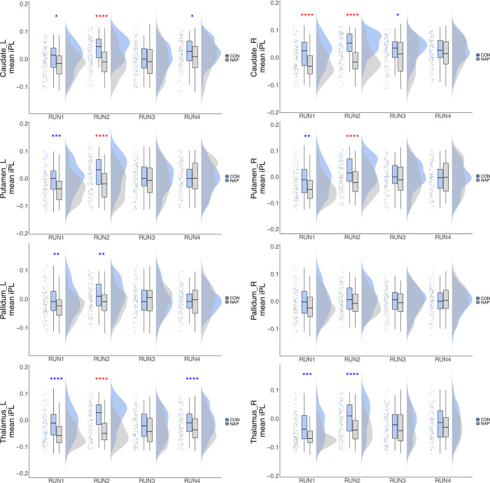
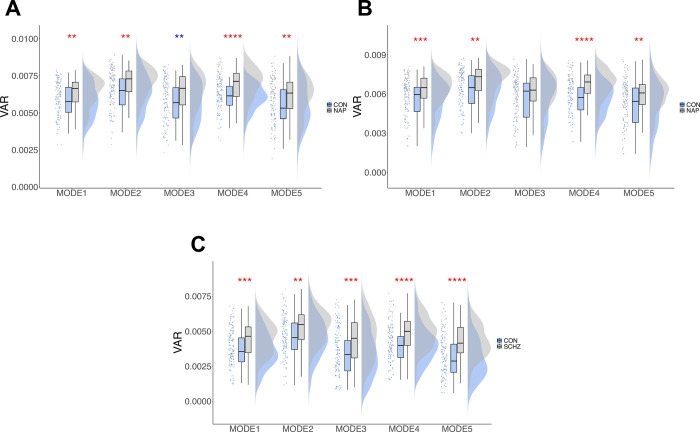
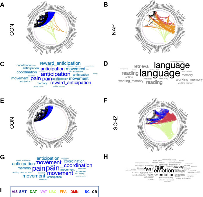
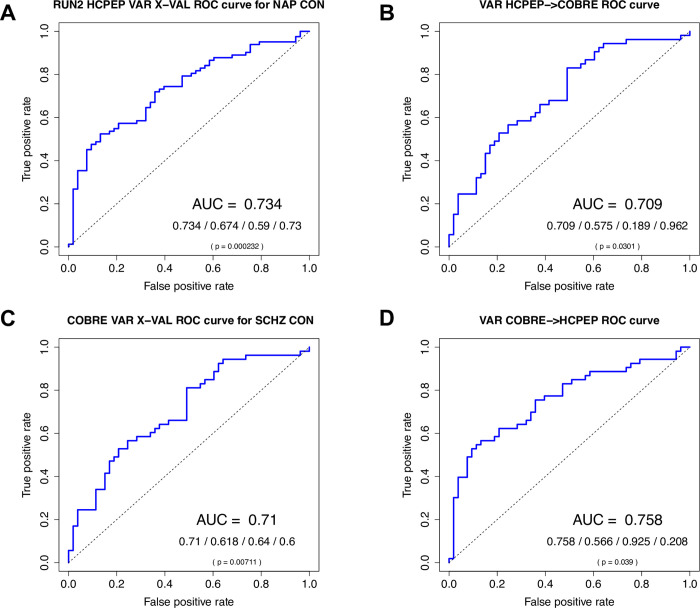
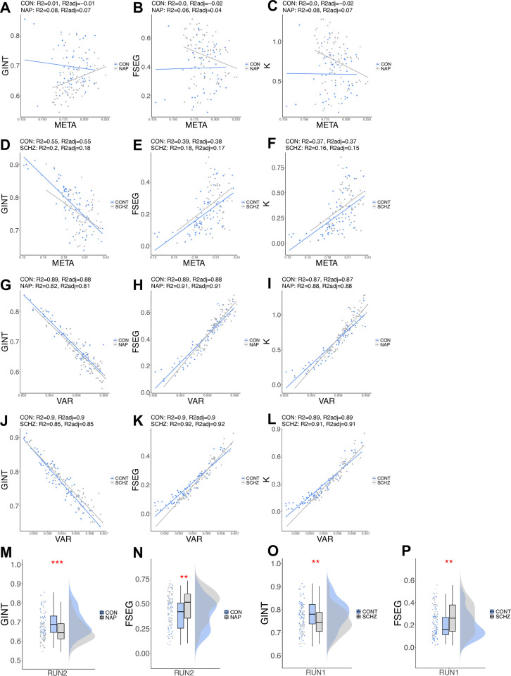
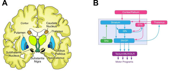
The disconnection hypothesis of schizophrenia proposes that symptoms of the disorder arise as a result of aberrant functional integration between segregated areas of the brain. The concept of metastability characterizes the coexistence of competing tendencies for functional integration and functional segregation in the brain, and is therefore well suited for the study of schizophrenia. In this study, we investigate metastability as a candidate neuromechanistic biomarker of schizophrenia pathology, including a demonstration of reliability and face validity. Group-level discrimination, individual-level classification, pathophysiological relevance, and explanatory power were assessed using two independent case-control studies of schizophrenia, the Human Connectome Project Early Psychosis (HCPEP) study (controls n = 53, non-affective psychosis n = 82) and the Cobre study (controls n = 71, cases n = 59). In this work we extend Leading Eigenvector Dynamic Analysis (LEiDA) to capture specific features of dynamic functional connectivity and then implement a novel approach to estimate metastability. We used non-parametric testing to evaluate group-level differences and a naïve Bayes classifier to discriminate cases from controls. Our results show that our new approach is capable of discriminating cases from controls with elevated effect sizes relative to published literature, reflected in an up to 76% area under the curve (AUC) in out-of-sample classification analyses. Additionally, our new metric showed explanatory power of between 81-92% for measures of integration and segregation. Furthermore, our analyses demonstrated that patients with early psychosis exhibit intermittent disconnectivity of subcortical regions with frontal cortex and cerebellar regions, introducing new insights about the mechanistic bases of these conditions. Overall, these findings demonstrate reliability and face validity of metastability as a candidate neuromechanistic biomarker of schizophrenia pathology.

Fig 1. Diversity of phase-locking behavior.

A) Time-series of mode eigenvectors from two subjects from the HCPEP dataset. Top panel shows phase-locking behavior. Middle panel shows instantaneous magnetization which is the ratio of in-phase to antiphase regions. Bottom panel shows the mode assigned to the timepoint from k-means clustering. Interesting behavior is indicated with numbered circles. B) Blow-outs for points 1 to 5. C) Legend for the numbered circles. MAG, magnetization; M, mode. Gray dotted line shows where phase-locking is equal to zero.

Fig 2. Spatial patterns of recurrent phase-locked connectivity in RUN3 for controls.

A) Phase-locking patterns for the 5 modes in sagittal view. B) Phase-locking patterns for the 5 modes in axial view. C) Respective FC presented as connectograms color-coded as in Yeo [63] with the addition of dark blue for subcortical regions, and black for cerebellar regions. In Mode ψ₁ all regions are aligned in-phase and so there is no antiphase connectivity. FC computed as the outer product of the leading eigenvector for each mode. D) Color coded legend for the Yeo resting-state networks, subcortical and cerebellar regions. VIS, Visual; SMT, Somatomotor; DAT, Dorsal attention; VAT, Ventral attention; LBC, Limbic; FPA, Frontal parietal; DMN, Default mode network; SC, Subcortical; CB, Cerebellar.

Fig 3. Group differences in regional contribution to the leading eigenvector for Mode ψ₄.

Regional contribution was calculated as the mean value of instantaneous phase-locking over time for a particular anatomical region of interest. Raincloud plots show from left to right scatter plot for the raw data, boxplots showing the median, upper and lower quartiles, upper and lower extremes, and the distributions of the raw data. iPL, instantaneous phase-locking, * = 0.05, ** = 0.01, *** = 0.001, ****<0.001. Red * effect size between groups greater than effect size between runs. Blue * effect size between groups less than largest effect size between runs.

Fig 4. Most significant group differences in local VAR in the modes for HCPEP and Cobre datasets.

Raincloud plots show from left to right the raw data, boxplots showing the median, upper and lower quartiles, upper and lower extremes, and the distributions of the raw data. A) HCPEP RUN1. B) HCPEP RUN2. C) Cobre dataset. * = 0.05, ** = 0.01, *** = 0.001, ****<0.001. Red * effect size between groups greater than effect size between runs. Blue * effect size between groups less than largest effect size between runs.

Fig 5. Connectograms and word clouds for Mode ψ₄ in RUN2.

A) Group-level FC in Mode ψ₄ for HCPEP controls. B) Group-level FC in Mode ψ₄ for HCPEP Non-affective psychosis. C) The word cloud presents the top terms derived from Neurosynth using reverse inference for the regions in Mode ψ₄ for HCPEP controls. Word size represents the strength of the probabilistic association of the term to the regions. D) Top terms for Mode ψ₄ in HCPEP Non-affective psychosis. E) Group-wide FC in Mode ψ₄ for Cobre controls. F) Group-wide FC in Mode ψ₄ for Cobre Schizophrenia. G) Top terms for Mode ψ₄ in Cobre controls. H) Top terms for Mode ψ₄ in Cobre Schizophrenia. I) Color coded legend for the Yeo resting-state networks, subcortical and cerebellar regions. VIS, Visual; SMT, Somatomotor; DAT, Dorsal attention; VAT, Ventral attention; LBC, Limbic; FPA, Frontal parietal; DMN, Default mode network; SC, Subcortical; CB, Cerebellar.

Fig 6. naïve Bayes classifier results for discriminating cases from controls using a single a-priori feature VAR in Mode ψ₄.

A) Results for HCPEP model trained and cross-validated in RUN2. B) Results for HCPEP model trained and cross-validated in RUN2 and tested in Cobre. C) Results for Cobre model trained and cross-validated. D) Results for Cobre model trained and cross-validated in Cobre and tested in HCPEP RUN2. AUC/Balanced accuracy/Sensitivity/Specificity; p value calculated from the binomial distribution. AUC, area under receiver operating characteristic curve.

Fig 7. Time-series for the relative phase order and the Kuramoto order parameter for one NAP subject.

A) Time-series for the cosine of relative phase or instantaneous phase-locking for a single subject. B) Time-series for the Kuramoto order parameter or average phase for a single subject. C) Blow-outs showing how relative phase is more informative than average phase for the dynamics of brain activity in one subject. MAG, magnetization ratio; KOP, Kuramoto order parameter, CHI, chimerality.

Fig 8. Relationship between VAR and META with metrics of global integration, functional segregation, and a metastability index K.

A) HCPEP global integration versus META. B) HCPEP functional segregation versus META. C) HCPEP Metastability Index versus META. D) Cobre global integration versus META. E) Cobre functional segregation versus META. F) Cobre Metastability Index versus META. G) HCPEP global integration versus VAR. H) HCPEP functional segregation versus VAR. I) HCPEP Metastability Index versus VAR. J) Cobre global integration versus VAR. K) Cobre functional segregation versus VAR. L) Cobre Metastability Index versus VAR. R2 and R2adj results from linear regression. M) HCPEP Group-level differences in global integration. N) HCPEP Group-level differences in functional segregation. O) Cobre Group-level differences in global integration. P) Cobre Group-level differences in functional segregation. GINT, global integration; FSEG, functional segregations; K, Metastability Index.

Fig 9. Simple scheme of basal ganglia connectivity.

A) Location of the basal ganglia in an axial cartoon view of the brain. B) Basal ganglia connectivity. Arrows indicate direction of connectivity. Glutamatergic (Glu) structures are shown in rose, GABAergic nuclei are shown in cyan, and the dopaminergic (DA) nucleus is shown in green. STN, subthalamic nucleus; SNC, substantia nigra pars compacta; GPe, global pallidus external; GPi, global pallidus internal; SNr, Substantia nigra; MLR, midbrain locomotor region; diencephalon locomotor region.

Fig 10. Attractor landscape for the extended HKB model of multi-adic coordination.

A plot of the relative phase potential function landscape for A_ij = 2B_ij = 1 for each i, j. Note the many valleys (marked with red asterisks) in which an oscillator moving around in this landscape will become trapped. These valleys are the local minima corresponding to the coordination states. There are two types of valleys in this landscape: in-phase valleys, which have relatively very deep and wide basins of attraction, and antiphase valleys, which are narrower and shallower, reflecting the fact that the in-phase state is more stable than the antiphase state. Each of these valleys is separated by a distance of Π, and repeats infinitely on the potential surface in a 2 Π -periodic pattern. A, B, effective coupling parameters; i,j, i^th and j^th oscillator. Reproduced with permission from [52].

Fig 11. Statistical flowchart for non-parametric testing of differences between groups across runs.

1) 2x4 non-parametric ANOVA using Align rank transform (ART). 2) Friedmann repeated measures test. 3) Paired Wilcoxon test. 4) Friedmann repeated measures test. 5) Paired Wilcoxon test. 6) Independent Wilcoxon test for each run. 7) Independent Wilcoxon test across all runs.

References

1. Jongsma HE, Turner C, Kirkbride JB, Jones PB. International incidence of psychotic disorders, 2002–17: a systematic review and meta-analysis. Lancet Public Health. 2019. May 1;4(5):e229–44. doi: 10.1016/S2468-2667(19)30056-8 - DOI - PMC - PubMed
1. Bleuler E. Dementia praecox or the group of schizophrenias. Oxford, England: International Universities Press; 1950. 548 p. (Dementia praecox or the group of schizophrenias).
1. McCutcheon RA, Reis Marques T, Howes OD. Schizophrenia—An Overview. JAMA Psychiatry. 2020. Feb 1;77(2):201–10. doi: 10.1001/jamapsychiatry.2019.3360 - DOI - PubMed
1. Fusar‐Poli P, McGorry PD, Kane JM. Improving outcomes of first-episode psychosis: an overview. World Psychiatry. 2017;16(3):251–65. doi: 10.1002/wps.20446 - DOI - PMC - PubMed
1. Friston KJ. The disconnection hypothesis. Schizophr Res. 1998. Mar 10;30(2):115–25. doi: 10.1016/s0920-9964(97)00140-0 - DOI - PubMed
Publication types