A novel statistical methodology for quantifying the spatial arrangements of axons in peripheral nerves

Abstract

A thorough understanding of the neuroanatomy of peripheral nerves is required for a better insight into their function and the development of neuromodulation tools and strategies. In biophysical modeling, it is commonly assumed that the complex spatial arrangement of myelinated and unmyelinated axons in peripheral nerves is random, however, in reality the axonal organization is inhomogeneous and anisotropic. Present quantitative neuroanatomy methods analyze peripheral nerves in terms of the number of axons and the morphometric characteristics of the axons, such as area and diameter. In this study, we employed spatial statistics and point process models to describe the spatial arrangement of axons and Sinkhorn distances to compute the similarities between these arrangements (in terms of first- and second-order statistics) in various vagus and pelvic nerve cross-sections. We utilized high-resolution transmission electron microscopy (TEM) images that have been segmented using a custom-built high-throughput deep learning system based on a highly modified U-Net architecture. Our findings show a novel and innovative approach to quantifying similarities between spatial point patterns using metrics derived from the solution to the optimal transport problem. We also present a generalizable pipeline for quantitative analysis of peripheral nerve architecture. Our data demonstrate differences between male- and female-originating samples and similarities between the pelvic and abdominal vagus nerves.

Keywords: Sinkhorn distance; neuroanatomy; neuromodulation; optimal transport problem; peripheral nervous system; spatial point process.

Figure 1

The pipeline for the quantitative analysis of the spatial arrangement of axons in the peripheral nerve cross-sections.

Figure 2

(A, D) The transmission electron microscopy (TEM) images of the nerve cross-section of Image 15 (vagus) and Image 29 (pelvic) listed in Table 1, respectively. The visible void spaces in the nerve cross-sections are blood vessels. The tiny light gray regions without any border are the unmyelinated axons. The myelinated axons have slightly darker gray borders. (B, E) The automated segmentation of the unmyelinated axons (the white regions) in the nerve cross-sections. (C, F) The spatial point patterns constructed with the centroid locations (the black circles) of the segmented unmyelinated axons.

Figure 3

An illustration of spatial point patterns with different spatial intensities. Samples 1, 2, and 3 have 20, 100, and 200 points per unit area, respectively.

Figure 4

An illustration of spatial point patterns with different spatial interactions. (A) SPPs portraying complete spatial randomness (sample 1), spatial inhibition (sample 2), and spatial attraction (sample 3). (B) Besag's centered L-function computed for the patterns shown in (A). The solid lines illustrate the spatial interaction of the patterns compared to CSR. The shaded area around the solid lines shows the boundaries of 95-percentile confidence interval.

Figure 5

Besag's centered inhomogeneous L-function computed for Images 15 and 29. The shaded area around L(r) = 0 shows the significance bands of complete spatial randomness (CSR). The solid lines illustrate the non-random spatial arrangement of the point patterns compared to CSR. The shaded area around the solid lines shows the boundaries of 95-percentile confidence interval.

Figure 6

(A) Inhomogeneous random spatial point patterns with no directional preference (Sample 1), horizontal (Sample 2), and vertical (Sample 3) directional preferences. (B) Differences computed between the horizontal and vertical K-functions for the samples in (A).

Figure 7

An illustration of spatial point patterns with different inhomogeneous spatial interactions. (A) Spatial inhibition. (B) Spatial randomness. (C) Spatial clustering. The intensity functions of the random and clustered patterns introduce some anisotropy. (D) An embedding of the point patterns in the Sinkhorn space. The inhibited, random, and clustered point patterns are shown in green, blue, and orange, respectively.

Figure 8

An illustration of spatial point patterns with different interactions and regionality. (A) Simulated examples of spatial point patterns: concentrated in the upper right (1, 2, 5, 6, 9, 10, 13, 14) and the lower left (3, 4, 7, 8, 11, 12, 15, 16) corners demonstrate regionality. The points are organized randomly in the odd-numbered examples and clustered in the even-numbered instances. (B) Euclidean distance between the inhomogeneous L-functions of the simulated models. (C) Sinkhorn distance between the local inhomogeneous L-functions of the simulated examples at a large interaction distance (r = 0.679). (D) Sinkhorn distance between the first principal component (PC) of local inhomogeneous L-functions of the simulated examples over a set of interaction distances. The point patterns of different interactions and regionality are shown in different colors.

Figure 9

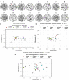
(A, C–I) A set of images of the segmented unmyelinated axons in the nerve cross-sections, labeled with the Image ID. (B) An embedding of the spatial intensity of the spatial point patterns in the Sinkhorn space for entropic regularization parameter λ = 0.01. The vagus and the pelvic samples are shown in cyan and orange [circles for female (F) and triangles for male (M)], respectively, and labeled with the Image ID listed in Table 1.

Figure 10

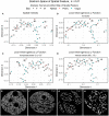
(A, B) The segmented unmyelinated axons and the spatial point pattern of Image 18 (vagus) listed in Table 1. (C–E) The embeddings of the local inhomogeneous and anisotropic L-functions (no sector, horizontal sector, and vertical sector) of the spatial point patterns in the Sinkhorn space for entropic regularization parameter λ = 0.01. The vagus and the pelvic samples are shown in cyan and orange [circles for female (F) and triangles for male (M)], respectively, and labeled with the Image ID listed in Table 1.

Figure 11

Visualizing the kernel-smoothed spatial features of Image 3 (vagus) and Image 29 (pelvic) listed in Table 1. (A, E) Spatial intensity. (B, F) Local inhomogeneous L-function. (C, G) Local inhomogeneous L-function with the horizontal sector. (D, H) Local inhomogeneous L-function with the vertical sector. The scale bars show the range of values for each spatial feature separately (column-wise). The kernel-smoothed bitmaps were downsampled for reasonable runtime and memory requirements.

Figure 12

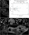
(A–D) The embeddings of the kernel-smoothed spatial intensity and the local inhomogeneous and anisotropic L-functions (no sector, horizontal sector, and vertical sector) of the spatial point patterns in the Sinkhorn space for entropic regularization parameter λ = 0.01. The vagus and the pelvic samples are shown in cyan and orange [circles for female (F) and triangles for male (M)], respectively, and labeled with the Image ID listed in Table 1. (E–H) The segmented unmyelinated axons of Image 15 and 6 (vagus) and Image 19 and 26 (pelvic) listed in Table 1.

Figure 13

Boxplots displaying the ranges of Sinkhorn distance between the spatial intensity of the nerve cross-sections. Pelv: pelvic; Vag: vagus. (A) Analysis of the spatial point patterns directly. (B) Analysis of the kernel-smoothed maps of the spatial features. The points show the individual Sinkhorn distances, revealing the hidden distribution.

Figure 14

Boxplots displaying the ranges of Sinkhorn distance between the spatial intensity of the sub-categories of the nerve cross-sections. Abd: abdominal vagus; Cerv: cervical vagus, and pelvic. (A, B) Analysis of the spatial point patterns directly. (C, D) Analysis of the kernel-smoothed maps of the spatial features. The points show the individual Sinkhorn distances, revealing the hidden distribution.

References

1. Ahuja R. K., Magnanti T. L., Orlin J. B. (1993). Network Flows - Theory, Algorithms and Applications. Prentice Hall.
1. Asala S. A., Bower A. J. (1986). An electron microscope study of vagus nerve composition in the ferret. Anat. Embryol. 175, 247–253. 10.1007/BF00389602 - DOI - PubMed
1. Avis D. (1980). On the extreme rays of the metric cone. Can. J. Math. 32, 126–144. 10.4153/CJM-1980-010-0 - DOI
1. Baddeley A., Rubak E., Turner R. (2015). Spatial Point Patterns: Methodology and Applications With R. London: Chapman and Hall; CRC Press. 10.1201/b19708 - DOI
1. Baddeley A. J., Møller J., Waagepetersen R. (2000). Non- and semi-parametric estimation of interaction in inhomogeneous point patterns. Stat. Neerland. 54, 329–350. 10.1111/1467-9574.00144 - DOI
LinkOut - more resources