The color of environmental noise in river networks

Abstract

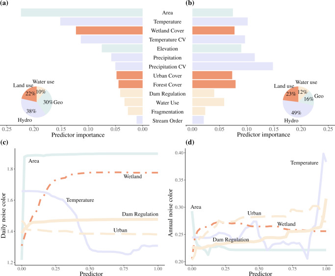
Despite its far-reaching implications for conservation and natural resource management, little is known about the color of environmental noise, or the structure of temporal autocorrelation in random environmental variation, in streams and rivers. Here, we analyze the geography, drivers, and timescale-dependence of noise color in streamflow across the U.S. hydrography, using streamflow time series from 7504 gages. We find that daily and annual flows are dominated by red and white spectra respectively, and spatial variation in noise color is explained by a combination of geographic, hydroclimatic, and anthropogenic variables. Noise color at the daily scale is influenced by stream network position, and land use and water management explain around one third of the spatial variation in noise color irrespective of the timescale considered. Our results highlight the peculiarities of environmental variation regimes in riverine systems, and reveal a strong human fingerprint on the stochastic patterns of streamflow variation in river networks.

Fig. 1. Observed patterns of flow noise color across 7504 (for daily data) and 2594 stream gages (for annual data) across the conterminous United States.

In a and b we show the spatial distribution of daily and annual flow noise color respectively, together with their density distributions (for annual flow noise color, we show the mean, minimum, and maximum annual flow; obtained from the average, minimum, and maximum daily flows in a year). Four different sites are shown, selected to illustrate a range of flow regimes: site 1, USGS gage #08086212, Hubbard Creek in Albany, Texas (white daily and annual noise color); site 2, USGS gage #12178100, Newhalem Creek in Washington (pink daily and blue annual noise color); site 3, USGS gage #10255550, New River in Westmorland, California (red daily and pink annual noise color); and site 4, USGS gage #02228000, Satilla River in Atkinson, Georgia (black daily and white annual noise color). The background of the CONUS credits to Copyright:© 2013 National Geographic Society, i-cubed in ArcGIS® software by Esri.

Fig. 2. Observed flow regimes and noise color at daily and annual scales.

In a and b we show hydrographs, Autocorrelation Functions (ACF), and spectral density plots for four different sites (shown in Fig. 1), calculated based on daily flow values (a), and mean annual flow values (b). The spectral density plots show how noise color is calculated from the linear regression of spectral density against frequency (noise color is the slope in opposite sign; see Eq. 3 in Methods). Warmer colors indicate higher ‘memory’–as indicated by significant correlation at longer lags.

Fig. 3. Environmental and human-related drivers of flow noise color.

Relative importance of natural and anthropogenic drivers of flow noise color at the daily scale (a) and at the annual scale (b); and partial dependence plots of 5 selected drivers on daily noise color (c) and annual noise color (d). Partial dependence plots (c, d) show change in noise color attributed to each variable while removing the influence of other variables. The x-axes in c, d represent the dimensionless scales of the variables after normalizing them between 0 and 1. The color of bars in a, b indicate the different driver categories: hydroclimate (Hydro), geography (Geo), land use – land cover (Land use), and human activities on the water cycle (Water management, indicated as Water use). The relative importance of each driver was evaluated using random forest models (see Methods for model details), and is illustrated via pie charts by driver category.

Fig. 4. Flow noise color predicted by the random forest models at ~430,000 river reaches (~1.9 million km) across U.S. river networks.

a Daily flow noise color; b Annual flow noise color. In c, d we show predicted daily and annual flow noise color for river basins in the U.S. Southeast. The contour of the CONUS credits to Copyright:© 2013 National Geographic Society, i-cubed in ArcGIS® software by Esri.

References

1. Sabo JL, Post DM. Quantifying periodic, stochastic, and catastrophic environmental variation. Ecol. Monogr. 2008;78:19–40. doi: 10.1890/06-1340.1. - DOI
1. Schwager M, Johst K, Jeltsch F. Does red noise increase or decrease extinction risk? Single extreme events versus series of unfavorable conditions. Am. Naturalist. 2006;167:879–888. doi: 10.1086/503609. - DOI - PubMed
1. Halley, J. M. Ecology, evolution and 1/f-noise. Trends Ecol. Evol. 10.1016/0169-5347(96)81067-6 (1996). - PubMed
1. Vasseur DA, Yodzis P. The color of environmental noise. Ecology. 2004;85:1146–1152. doi: 10.1890/02-3122. - DOI
1. Kroeker KJ, et al. Ecological change in dynamic environments: accounting for temporal environmental variability in studies of ocean change biology. Glob Change Biol. 2020;26:54–67. doi: 10.1111/gcb.14868. - DOI - PubMed