Foundation model of neural activity predicts response to new stimulus types and anatomy

Abstract

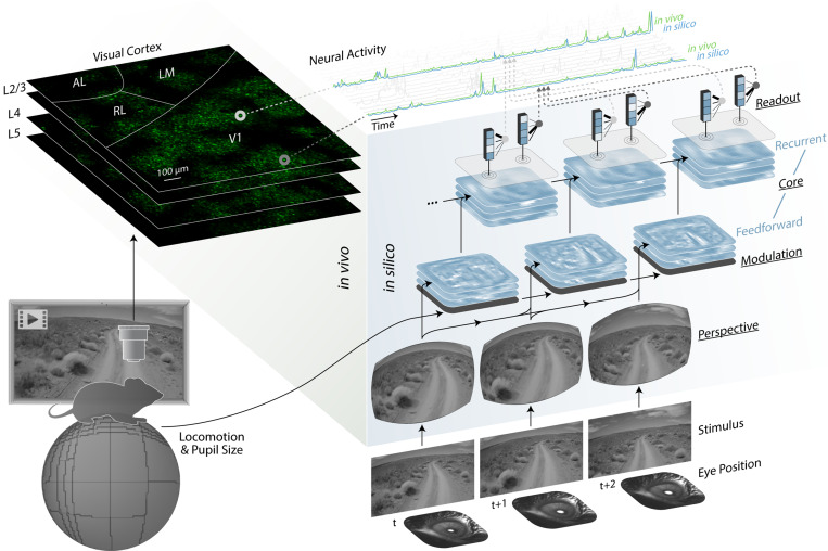
The complexity of neural circuits makes it challenging to decipher the brain's algorithms of intelligence. Recent breakthroughs in deep learning have produced models that accurately simulate brain activity, enhancing our understanding of the brain's computational objectives and neural coding. However, these models struggle to generalize beyond their training distribution, limiting their utility. The emergence of foundation models, trained on vast datasets, has introduced a new AI paradigm with remarkable generalization capabilities. We collected large amounts of neural activity from visual cortices of multiple mice and trained a foundation model to accurately predict neuronal responses to arbitrary natural videos. This model generalized to new mice with minimal training and successfully predicted responses across various new stimulus domains, such as coherent motion and noise patterns. It could also be adapted to new tasks beyond neural prediction, accurately predicting anatomical cell types, dendritic features, and neuronal connectivity within the MICrONS functional connectomics dataset. Our work is a crucial step toward building foundation brain models. As neuroscience accumulates larger, multi-modal datasets, foundation models will uncover statistical regularities, enabling rapid adaptation to new tasks and accelerating research.

Keywords: Artificial Intelligence; Foundation model; Generalization; Visual cortex.

Extended Data Fig. 1.. ANN perspective.

Schematic of the modeled perspective the animal. a, The retina is modeled as points on a sphere receiving light rays that trace through the origin. An example light ray with polar angle $\theta$ and azimuthal angle $\varphi$ is shown in red. b, The light ray is traced to a point $m^x,m^y$ on the monitor. Bilinear interpolation of the four pixels on the monitor surrounding $m^x,m^y$ produces the activation of a point $\theta ,\varphi$ on the modeled retina. c, 9 examples of the modeled perspective from the left eye of an animal, with 3 horizontal rotations of the optical globe (abduction/adduction) × 3 vertical rotations (elevation/depression). The concentric circles indicate visual angles in degrees. (See Methods for details on the perspective network.)

Extended Data Fig. 2.. ANN modulation.

Visualization of the modulation network’s output, projected onto 2 dimensions via UMAP. a, b show the same data from an example recording session and modulation network. Each point on the plot indicates a point in time from the recording session. The colors indicate measurements of pupil size (a) and treadmill speed (b) at the respective points in time. (See Methods for details on the modulation network.)

Extended Data Fig. 3.. Neural network lesion studies.

To determine the effect that various components of the model have on predictive accuracy, we performed lesion studies, where we altered individual components of model and evaluated the effect that the alteration had on model performance $\left(C{C}_{abs}\right)$. The left 4 columns (a-d, f-i, k-n, p-s) are scatterplots of reference vs lesioned model performance, with each column corresponding to different mouse and each point corresponding to a neuron. The right-most column (e, j, o, t) displays density histograms of the performance difference between the reference and the lesioned models, plotted separately for each mouse, as well as the t-statistic and p-values of paired two-sided t-tests. The first row (a-e) shows the effect of the perspective module on model performance, the second row (f-j) shows the effect of the modulation module, the third row (k-o) shows the effect of the convolution type – 2D vs 3D – of the feedforward module, and the fourth row (p-t) shows the effect of the loss function – Poisson negative log likelihood (Poission NLL) vs mean square error (MSE).

Extended Data Fig. 4.. ANN performance: Individual vs. Foundation.

Predictive accuracy (median $C{C}_{norm}$ across neurons) of foundation models (with the foundation core) vs. individual models (with cores trained on individual recording sessions). For the 4 mice in the 4 left columns, 1 recording session was performed, and that data was partitioned into 7 training/validation splits, which were used to train separate individual/foundation models. The predictive accuracy of those models (diamonds) is reported for 6 testing stimulus domains (rows). For the MICrONS mouse, 14 recording sessions were performed, for each recording session, a model was trained using nearly all (99%) of the data available for training/validation. The MICrONS models were only tested on the natural movies, due to the lack of the other stimuli in the recording sessions. All models were trained only using natural movies.

Extended Data Fig. 5.. Recurrent architecture: Conv-Lstm vs. CvT-Lstm.

We evaluated the performance of two different types of recurrent architectures for the core module: Conv-Lstm (blue) and CvT-Lstm (tan). For each architecture, a core was trained on 8 mice and then transferred to 4 new mice. For each of the new mice, 7 models were trained using varying amounts of natural movies, ranging from 4 to 76 minutes. The predictive accuracy $\left(C{C}_{norm}\right)$ of these models was evaluated on 6 different stimulus domains: natural movies (a), natural images (b), drifting gabor filter (c), flashing Gaussian dots (d), directional pink noise (e), random dot kinematograms (f). Blue diamonds indicate models with the Conv-Lstm core, and tan diamonds indicate models with the CvT-Lstm core. For each architecture, models of the same mouse are connected by lines.

Extended Data Fig. 6.. Reliability of in vivo and in silico direction and orientation tuning.

a: Direction selectivity index (DSI) of neurons measured in two different in vivo experiments (i.e., recording sessions). Each point represents a single neuron measured in the two in vivo experiments. b: DSI measured in two different in silico experiments (i.e., model of a recording session). Each point represents a single neuron measured in the two in silico experiments. c: Distribution of the absolute differences between two measurements of DSI from in vivo (dashed) and insilico (solid) experiments. d-f: Same as a-c, but for orientation selectivity index (OSI). g-i: Same as a-c, but for preferred direction. j-l: Same as a-c, but for preferred orientation.

Extended Data Fig. 7.. Pairwise similarities of readout feature weights of neurons from the MICrONS volume.

Here we examine the similarities of readout weights of same or different neurons, from same or different scans (recording sessions). In panels a–c, the similarities of readout weights are plotted for the following groups: same neuron from different scan (y-axis of a), same neuron from same scan (y-axis of b), different neuron from different scan (x-axis of a, x-axis of c), different neuron from same scan (x-axis of b and y-axis of c). The similarity between readout weights was measured inversely via angular distance $\angle :=\arccos ((x\cdot y)/(\parallel x\parallel \parallel y\parallel ))/\pi$, where $\mathbf{\text{x}}$, $\mathbf{\text{y}}$ is a pair of readout weights. A similar pair of readout weights will exhibit a small $\angle$, and vice versa. The scatterplots a–c are colored by the $C{C}_{\max }$, which is an inverse measure of neuronal noise, i.e., the estimated maximum correlation coefficient that a model could achieve at predicting the mean response the neuron (see Methods for details). For each neuron N, the “different” neuron N’ was restricted to be $\le 100\text{μm}$ apart from each other in terms of soma distance, and the distribution of the number of “different” neurons is shown in d (from different scans) and e (from the same scan). f and g (corresponding to d and e, respectively) show the fraction of the nearby neurons N’ that are more similar to N in terms of readout weights than N is to itself across different scans. f, For 919 out of the 1013 neurons N, less than 0.05 of nearby neurons N’ from different scans had more similar readout weights. g, For 840 out of the 1013 neurons N, less than 0.05 of nearby neurons N’ from the same scan had more similar readout weights.

Fig. 1.. ANN model of the visual cortex.

The left panel (green) depicts an in vivo recording session of excitatory neurons from several areas (V1, LM, RL, AL) and layers (L2/3, L4, L5) of the mouse visual cortex. The right panel (blue) shows the architecture of the ANN model and the flow of information from inputs (visual stimulus, eye position, locomotion, and pupil size) to outputs (neural activity). Underlined labels denote the four main modules of the ANN: perspective, modulation, core, and readout. For the modulation and core, the stacked planes represent feature maps. For the readout, the blue boxes represent the core’s output features at the readout position of the neuron, and the fanning black lines represent readout feature weights. The top of the schematic displays the neural activity for a sampled set of neurons. For two example neurons, in vivo and in silico responses are shown (green and blue, respectively).

Fig. 2.. Predictive accuracy of models trained on individual recording sessions.

a, Predictive accuracy (median $C{C}_{\text{norm}}$ across neurons, see Methods for details) of our model vs. the previous state-of-the-art dynamic model of the mouse visual cortex by Sinz et al. (2018). We trained and tested our model on the same set of data from Sinz et al. (2018): V1 neuronal responses to natural movies from 3 mice. n = number of neurons per mouse. ** = paired two-way $t$-test, t=14.53, p < 0.01, df=2. b, Predictive accuracy of our models by the amount of data used for training for 4 new recording sessions and mice. For each recording session, training data was partitioned in to 7 fractions ranging from 4 to 76 minutes. Separate models (diamonds) were trained on the differing fractions of training data, but tested on the same held-out testing data. Models of the same mice are connected by lines. c, Predictive accuracy by visual area, from models that were trained on the full data. We did not find a statistically significant relationship between predictive accuracy and visual areas (linear mixed effects model (Lindstrom and Bates, 1988), n.s. = Wald test, p = 0.45, df=3).

Fig. 3.. Predictive accuracy of foundation models.

a, Schematic of the training and testing paradigm. Natural movie data were used to train: 1) a combined model of the foundation cohort of mice with a single foundation core, and 2) foundation models vs. individual models of new mice. The models of the new mice were tested with stimuli from 6 different domains (b’–g’). b–g, Corresponding plots show the predictive accuracy (median $C{C}_{\text{norm}}$ across neurons) as a function of the amount of training data for foundation models (blue) vs. individual models (gray) of the new mice. 4 mice × 7 partitions of training data × 2 types of models = 56 models (diamonds). Models of the same mouse and type (foundation / individual) are connected by lines. Number of neurons per mouse = 8,862 | 8,014 | 9,452 | 10,246.

Fig. 4.. Parametric tuning from the foundation model.

a, Schematic of the experimental paradigm: foundation models of new mice (n=3) were trained with natural movies, and estimates of parametric tuning were computed from in vivo and in silico responses to synthetic stimuli (b’, directional pink noise; c’, flashing Gaussian dots). b,c, In vivo and in silico estimates of an example neuron’s parametric tuning to orientation/direction (b) and spatial location (c). d,f,h, Binned scatter plots of in vivo and in silico estimates of selectivity indices (SI) for orientation (d, OSI), direction (f, DSI), and spatial (h, SSI). The color indicates the number of neurons (n) in each bin. e,g,i, Density histograms of differences between in vivo and in silico estimates of preferred orientation (e), direction (g), and spatial location (i). In each panel, histograms containing increasingly selective groups of neurons, thresholded by in silico OSI (e) / DSI (g) / SSI (i), are stacked from top to bottom. The density histograms were produced via kernel density estimation using Scott’s bandwidth.

Fig. 5.. The foundation model of the MICrONS volume relates neuronal function to structure and anatomy.

a, Schematic of a foundation model of the MICrONS mouse, trained on excitatory neuronal responses to natural movies. At the bottom, the readout at a single time point is depicted, showing the readout positions and feature weights for two example neurons. b, Meshes of two example neurons, reconstructed from serial electron microscopy. The zoom-in cutout shows a synapse between these two neurons, with the pre-synaptic axon in black and post-synaptic dendrite in silver. c, Colored scatter plots of readout positions of all neurons from a recording session of the MICrONS mouse, overlayed on top-down a view of the recording window with annotated visual areas (V1, LM, RL, AL) and boundaries. The left and right plots are colored by the $x$ and $y$ coordinates of the readout positions, respectively. d, Confusion matrix of MICrONS visual areas predicted from readout feature weights, normalized per row. The diagonal represents the recall for each visual area. e, Confusion matrix of MICrONS excitatory neuron cell types predicted from readout feature weights, normalized per row. The excitatory neuron cell types are from Schneider-Mizell et al. 2023. The diagonal represents the recall for each cell type. f, Morphologies of different types excitatory neurons. Two example neurons are shown for each excitatory neuron cell type.

References

1. Antolik J., Hofer S. B., Bednar J. A., and Mrsic-flogel T. D.. Model constrained by visual hierarchy improves prediction of neural responses to natural scenes. PLoS Comput. Biol., pages 1–22, 2016. - PMC - PubMed
1. Bakhtiari S., Mineault P, Lillicrap T., Pack C., and Richards B.. The functional specialization of visual cortex emerges from training parallel pathways with self-supervised predictive learning. Advances in Neural Information Processing Systems, 34:25164–25178,2021.
1. Bashiri M., Walker E., Lurz K.-K., Jagadish A., Muhammad T., Ding Z., Ding Z., Tolias A., and Sinz F.. A flow-based latent state generative model of neural population responses to natural images. Advances in Neural Information Processing Systems, 34, 2021.
1. Bashivan P., Kar K., and DiCarlo J. J.. Neural population control via deep image synthesis. Science (New York, N.Y.), 364(6439), 2019. ISSN 1095–9203. doi: 10.1126/science.aav9436. - DOI - PubMed
1. Batty E., Merel J., Brackbill N., Heitman A., Sher A., Litke A., Chichilnisky E. J., and Paninski L.. Multilayer network models of primate retinal ganglion cells. In Proceedings of the International Conference for Learning Representations (ICLR), 2017.
Publication types