Coupling radiative, conductive and convective heat-transfers in a single Monte Carlo algorithm: A general theoretical framework for linear situations

Abstract

It was recently shown that radiation, conduction and convection can be combined within a single Monte Carlo algorithm and that such an algorithm immediately benefits from state-of-the-art computer-graphics advances when dealing with complex geometries. The theoretical foundations that make this coupling possible are fully exposed for the first time, supporting the intuitive pictures of continuous thermal paths that run through the different physics at work. First, the theoretical frameworks of propagators and Green's functions are used to demonstrate that a coupled model involving different physical phenomena can be probabilized. Second, they are extended and made operational using the Feynman-Kac theory and stochastic processes. Finally, the theoretical framework is supported by a new proposal for an approximation of coupled Brownian trajectories compatible with the algorithmic design required by ray-tracing acceleration techniques in highly refined geometry.

Fig 1. Illustration of a conducto-convecto-radiative configuration.

The solid domain Ω_S is shown in gray, m fluid cavities ${\Omega }_{F_i}$ are shown in light blue, and the surrounding fluid cavity ${\Omega }_{F^{\infty }}$ is shown in dark blue. Radiation is present within the whole scene and the system is entirely semi-transparent. Conduction takes place only in solids.

Fig 2. Implementation example for the probabilization proposition in the case of a problem that is only time-dependent.

Fig 3. Illustration of the three possible realizations for ΘFi.

Each realization represents one of the three contributions that can be returned: initial temperature θ_I, a radiance temperature θ_R and a boundary temperature with the solid θ_S. The notation (., t) means that the temperature of the fluid is not dependent on the location in the cavity and that the probe can be positioned anywhere.

Fig 4. Illustration of four realizations of ΘS(x→,t)): An initial condition θ_I at point x→I, a radiance temperature θ_R at point (x→R,tR), a fluid temperature θ_F at time t_F and a temperature θ_D imposed at the boundary at point (y→D,tD).

For clarity, we represent only one fluid cavity.

Fig 5. Representation of three realizations of Θ_R: A radiance temperature imposed on the boundary θR,∂ΩR,u→R at point y→R (at this point, the boundary ∂Ω_R coincides with ∂Ω_S), a solid temperature θ_S at point x→S, and a fluid temperature θ_F.

We note ${\overrightarrow{\mathit{x}}}_A\equiv {\overrightarrow{\mathit{x}}}_S$ and $\theta ({\overrightarrow{\mathit{x}}}_A,t)\equiv {\theta }_S({\overrightarrow{\mathit{x}}}_S,t)$ if ${\overrightarrow{\mathit{x}}}_A\in {\Omega }_S$, and ${\overrightarrow{\mathit{x}}}_A\equiv {\overrightarrow{\mathit{x}}}_F$ and $\theta ({\overrightarrow{\mathit{x}}}_A,t)\equiv {\theta }_F({\overrightarrow{\mathit{x}}}_F,t)={\theta }_F(t)$ if ${\overrightarrow{\mathit{x}}}_A\in {\Omega }_F$. For clarity, we represent here only one fluid cavity.

Fig 6. Illustration of a realization of a recursive path starting from (x→,t) in the framework of model (6).

Information first spreads by conduction in the solid domain, until it reaches the fluid domain. Once in the fluid, it propagates by convection until it reaches the solid boundary at point $({\overrightarrow{\mathit{y}}}_{\mathit{S}}^{\mathit{F}},t_S^F)$. Back in the solid, information continues to spread by conduction until reaching a radiative source at $({\overrightarrow{\mathit{x}}}_{\mathit{R}}^{\mathit{S}},t_S)$. Then it propagates by radiation until being absorbed in the solid at point $({\overrightarrow{\mathit{x}}}_{\mathit{A}}^{\mathit{R}},t_S)$, before finally reaching by conduction the point $({\overrightarrow{\mathit{x}}}_{\mathit{I}},t_I)$ where temperature is known. Through this example recursive path, the contribution to temperature $\theta (\overrightarrow{\mathit{x}},t)$ is the initial condition ${\theta }_I({\overrightarrow{\mathit{x}}}_{\mathit{I}})$.

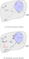
Fig 7

(a) matches Fig 6 for which only the points corresponding to the end of sub-paths (coupled propagators) are defined. (b) illustrates the whole path for each transfer mode, starting from the observation point $(\overrightarrow{\mathit{x}},t)$ until finding a prescribed temperature (here a temperature at the initial condition at ${\overrightarrow{\mathit{x}}}_{\mathit{I}})$. Brownian paths are black lines, radiative paths red lines and convective paths by blue dotted lines. The illustrated sequence is: conduction → convection → conduction → radiation → conduction. While only the beginning and the end of each sub-path is shown in (a), a detailled example of the sub-path for each transfer mode is displayed in (b). The standard illustration (see [117]) of the multi-scattering radiative path results from the iterative sampling of scattering free path lengths and propagation directions. (a) Green functions method and (b) Stochastic process method.

Fig 8. Illustration of thermal path sampling in a confined environment with a δ-sphere random walk for conductive paths.

The bidirectional arrows represent the fact that an intersection test must be performed in two opposite directions at each jump, in order to obtain the local δ step value. In red: the walking step is smaller than in the rest of the field, and the walk ends exactly at the boundary. At position ${\overrightarrow{\mathit{x}}}_2$ the conductive path switches to a radiative path until position ${\overrightarrow{\mathit{x}}}_3$.

Fig 9. Fig 7 is completed by the representation of a diffusive random walk under the approximation of a δ-sphere random walk.

(a) Green functions method, (b) Stochastic process method, and (c) Stochastic process method.

Fig 10. Illustration of methods based on Green’s function first-passage algorithms.

(a) WoS and (b) Walk-on-rectangle-parallelepiped.

Fig 11. Each θ_S and θ˜S curve are the exact solutions of respectively (83) and (84).

Points that are denoted MC and associated errorbars are the solutions of a numerical resolution by MC over the approximate model. The initial temperature field is: ${\theta }_I(\overrightarrow{\mathit{x}})={\theta }_{ref}+A\text{cos}(\overrightarrow{\mathit{k}}.\overrightarrow{\mathit{x}})$. Results have been obtained for a characteristic time τ and for position x ∈ [0, L], y = z = 0 with $\overrightarrow{\mathit{k}}=(2\pi /L,2\pi /L,2\pi /L)$, for each figure. The only differentiating parameter for the four figures is the value of δ that is taken respectively in the {L/2, L/5, L/10 and L/20} set. The scattering radiative coefficient is null (k_s = 0) and the reference temperature θ_ref that is used in coefficient ζ is chosen so that a equivalent weight is given to conduction and radiation, through the constraint $D||\overrightarrow{\mathit{k}}|{|}^2=\frac{\zeta k_a}{\rho C||\overrightarrow{\mathit{k}}||}arctan\left(\frac{||\overrightarrow{\mathit{k}}||}{k_e}\right)$. (a) δ = L/2, (b) δ = L/5, (c) δ = L/10, and (d) δ = L/20.

References

1. Kay TL, Kajiya JT. Ray tracing complex scenes. ACM SIGGRAPH computer graphics. 1986;20(4):269–278. doi: 10.1145/15886.15916 - DOI
1. Glassner AS. An introduction to ray tracing. Morgan Kaufmann; 1989.
1. Delatorre J, Baud G, Bézian JJ, Blanco S, Caliot C, Cornet JF, et al.. Monte Carlo advances and concentrated solar applications. Solar Energy. 2014;103:653–681. doi: 10.1016/j.solener.2013.02.035 - DOI
1. Villefranque N, Fournier R, Couvreux F, Blanco S, Cornet C, Eymet V, et al.. A Path-Tracing Monte Carlo Library for 3-D Radiative Transfer in Highly Resolved Cloudy Atmospheres. Journal of Advances in Modeling Earth Systems. 2019;11(8):2449–2473. doi: 10.1029/2018MS001602 - DOI
1. Fournier R, Blanco S, Eymet V, El Hafi M, Spiesser C. Radiative, conductive and convective heat-transfers in a single Monte Carlo algorithm. In: Journal of Physics: Conference Series. vol. 676. IOP Publishing; 2016. p. 012007.
Publication types
LinkOut - more resources