BICePs v2.0: Software for Ensemble Reweighting Using Bayesian Inference of Conformational Populations

Abstract

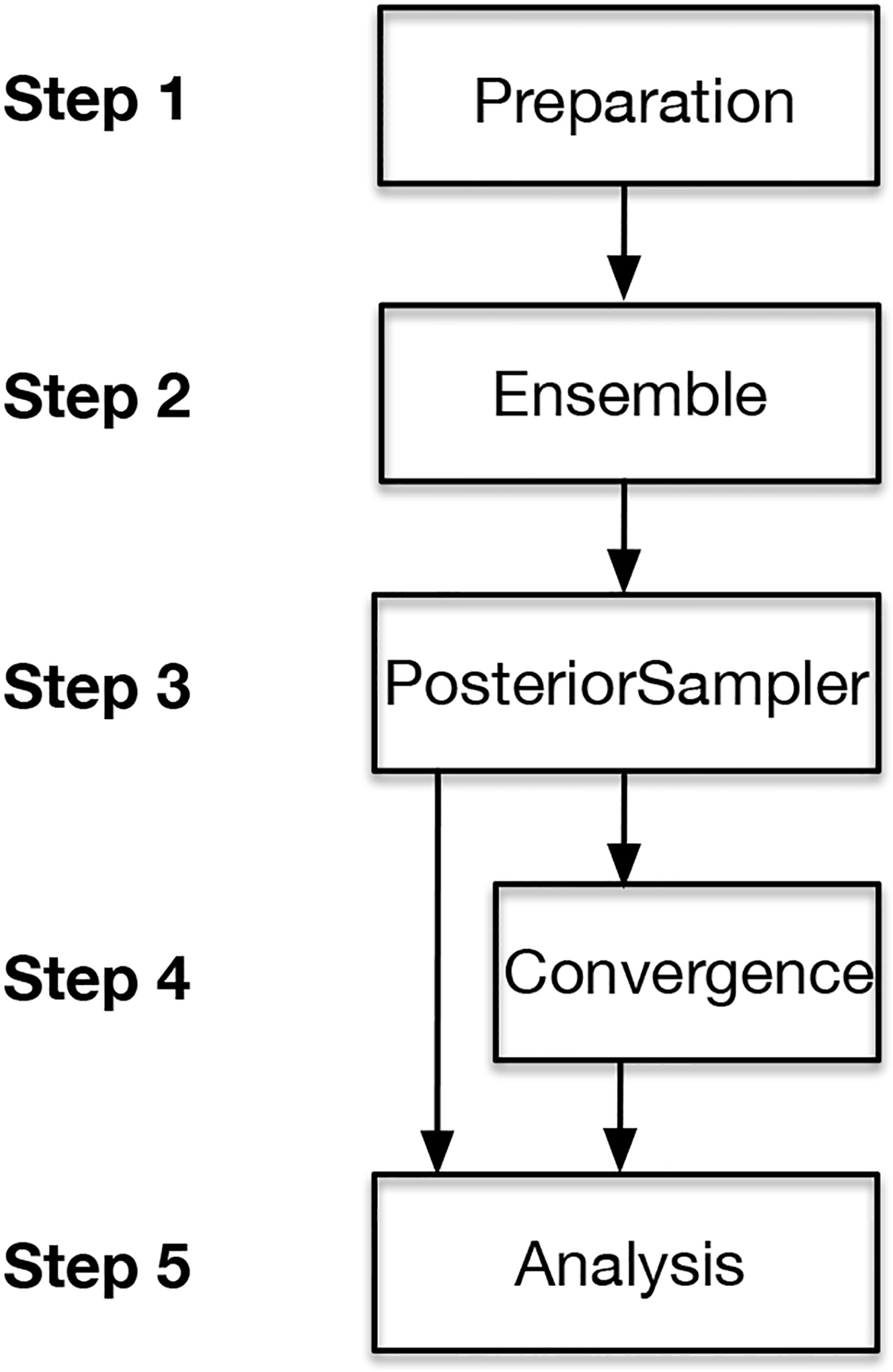
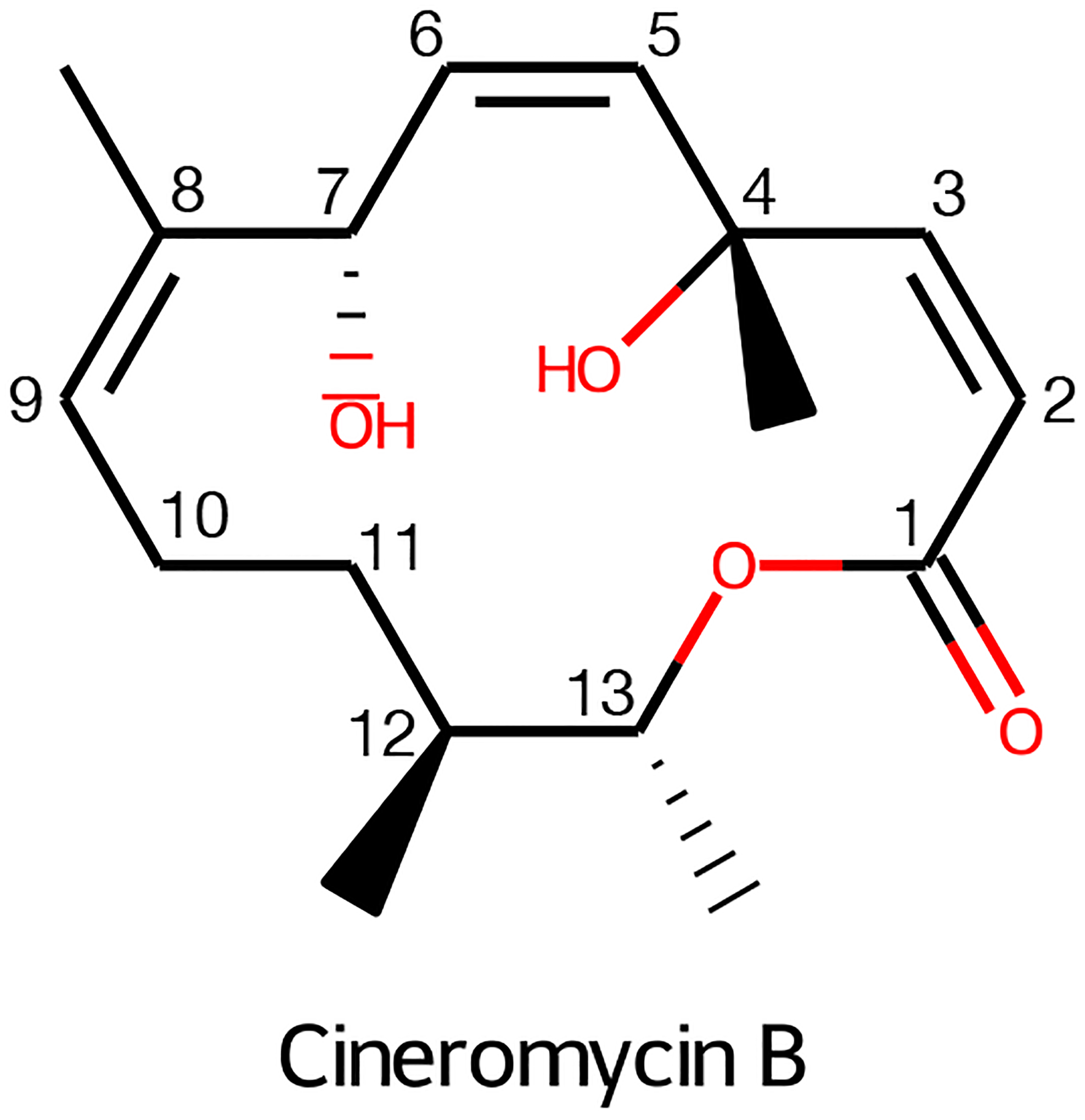
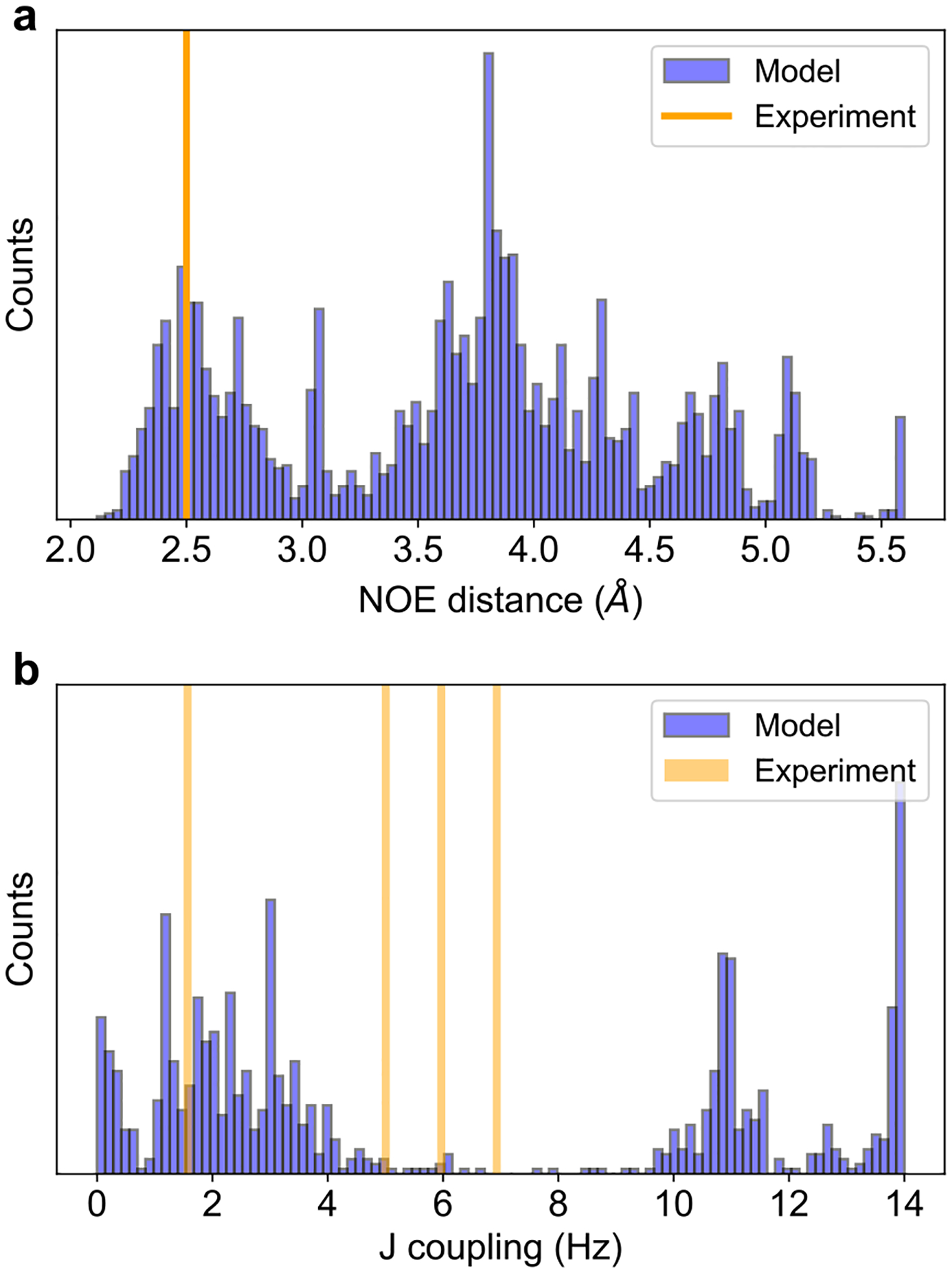
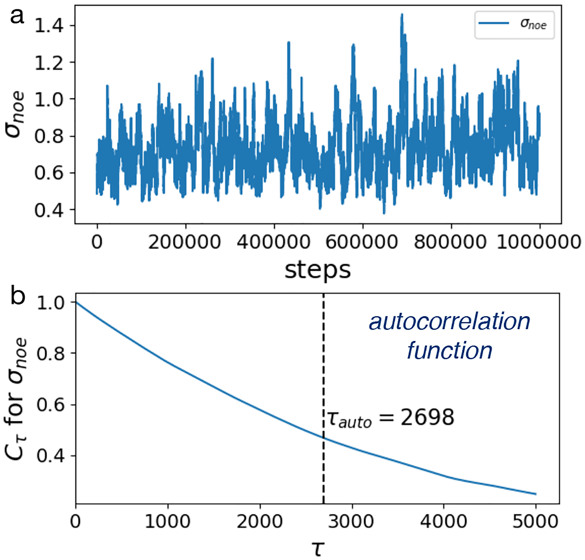
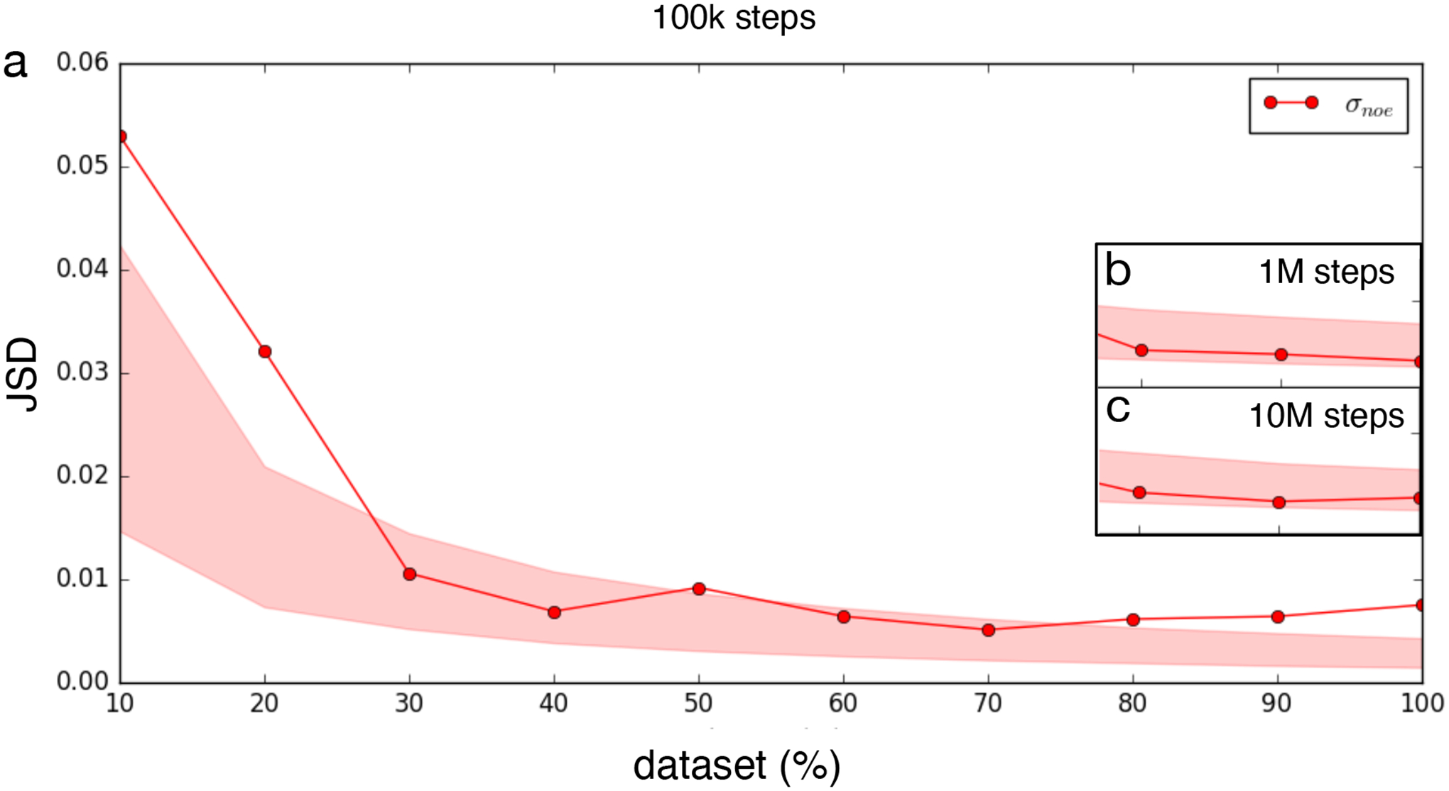
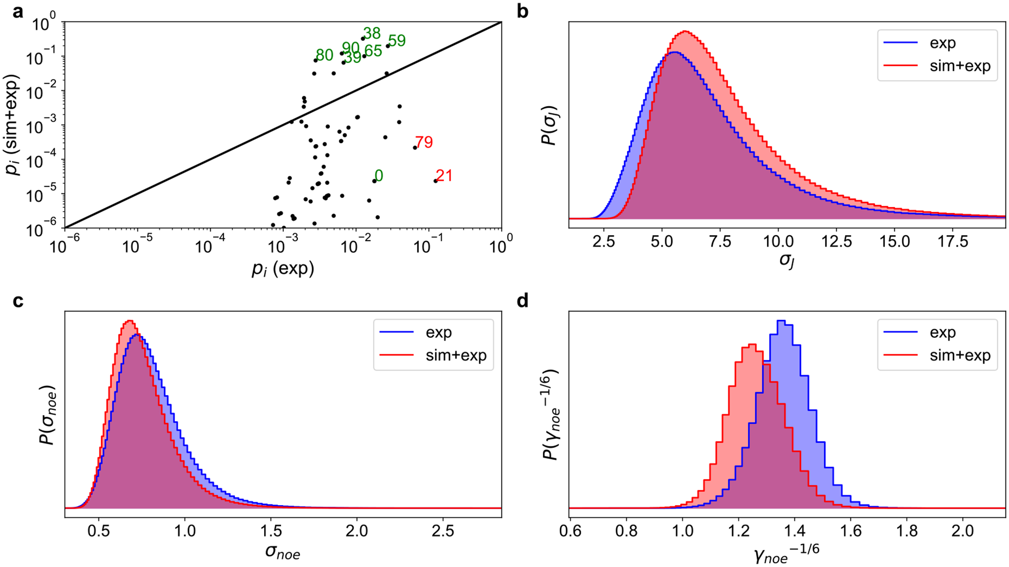
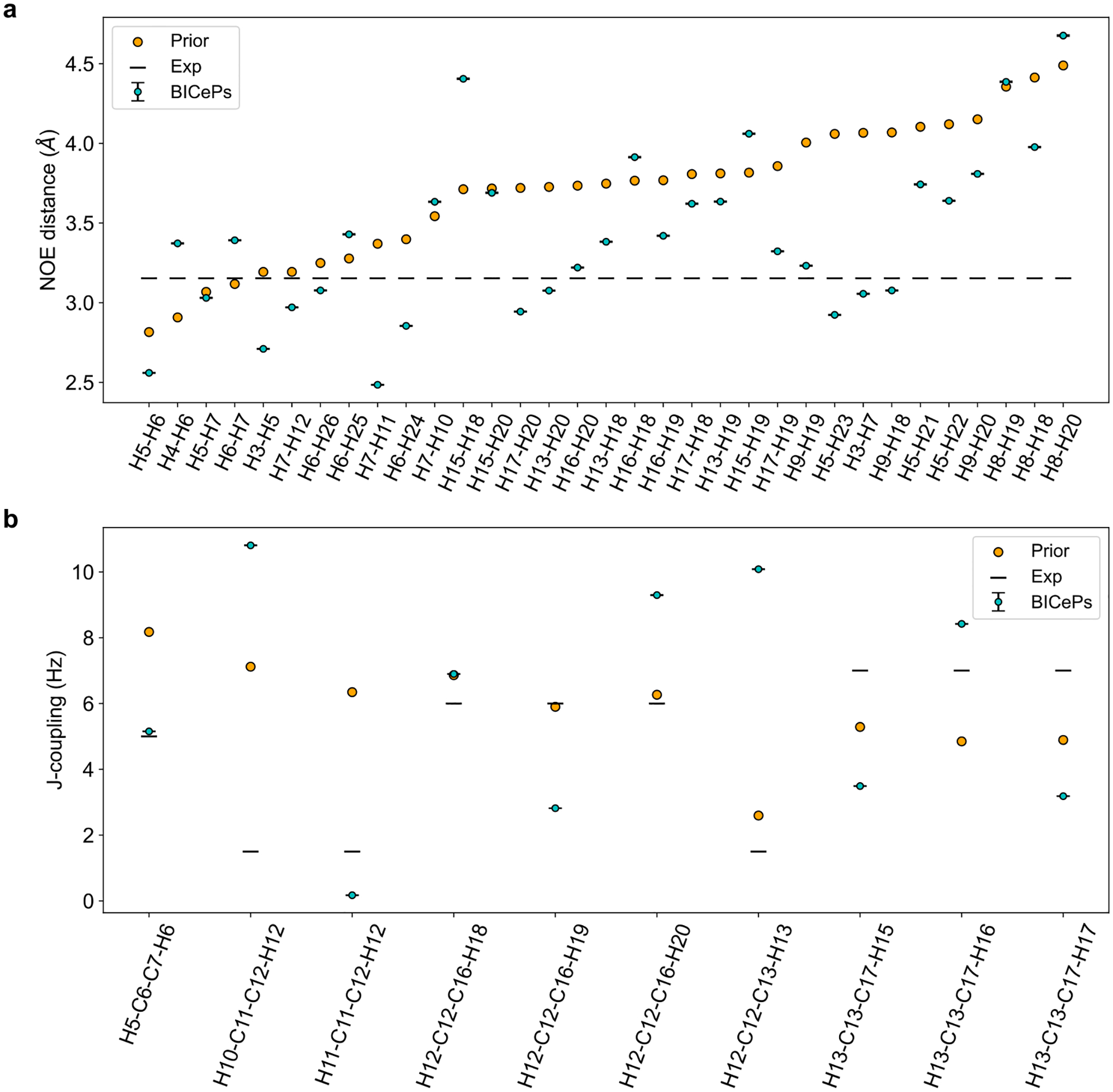
Bayesian Inference of Conformational Populations (BICePs) version 2.0 (v2.0) is a free, open-source Python package that reweights theoretical predictions of conformational state populations using sparse and/or noisy experimental measurements. In this article, we describe the implementation and usage of the latest version of BICePs (v2.0), a powerful, user-friendly and extensible package which makes several improvements upon the previous version. The algorithm now supports many experimental NMR observables (NOE distances, chemical shifts, J-coupling constants, and hydrogen-deuterium exchange protection factors), and enables convenient data preparation and processing. BICePs v2.0 can perform automatic analysis of the sampled posterior, including visualization, and evaluation of statistical significance and sampling convergence. We provide specific coding examples for these topics, and present a detailed example illustrating how to use BICePs v2.0 to reweight a theoretical ensemble using experimental measurements.

Figure 1:

The typical BICePs workflow.

Figure 2:

The line structure of the 14-membered macrocycle cineromycin B (7-O-demethylalbocycline).

Figure 3:

Histogram of experimental (orange) and model data (blue) for (a) 32 NOE distances, and (b) 9 scalar J-coupling observables, across all 100 conformational states of Cineromycin B.

Figure 4:

(a) Traces of ${\sigma }_{\text{NOE}}$ vs. MCMC sampling step during a BICePs calculation for the cineromycin B system. (b) Computed autocorrelation curve of the ${\sigma }_{\text{NOE}}$ trace for maxtau=5000.

Figure 5:

An example using Jensen-Shannon Divergence (JSD) analysis. (a) The JSD between the first and last half of the ${\sigma }_{\text{NOE}}$ trajectory, plotted as a function of the percentage of trajectory that has been sampled. The shaded region in this plot represents the 95% confidence interval of the JSD metric for the null distribution, calculated using a bootstrap procedure. (b-c) Extending the MCMC trajectories by 1M steps and 10M steps, respectively, results in the trajectory having complete statistical indistinguishability between the first and last halves.

Figure 6:

(a) A comparison of conformational state populations $p_i\left(\text{exp}\right)$ inferred using only experimental restraints, vs. BICePs populations $p_i\left(\text{sim}+\text{exp}\right)$ inferred using a combination of the simulation-based prior and experimental restraints. States on the lower right are highly compatible with experimental restraints, but are conformationally strained according to the simulation model. Conformational states near the top of the graph are both reasonably compatible with experimental restraints, and highly-populated according to the simulation model. (b) The marginal posterior distribution of ${\sigma }_{\text{J}}$, the uncertainty parameter for J-coupling constants. (c) The marginal posterior distribution of ${\sigma }_{\text{NOE}}$, the uncertainty parameter for NOE distance restraints. (d) The marginal posterior distribution of ${\gamma }_{\text{NOE}}$, the scaling parameter for the NOE distances, remains near 1.25 throughout the 100M steps of MCMC sampling.

Figure 7:

BICePs reweighted observables compared against experiment and prior for (a) NOE and (b) J-coupling. The error bars are calculated using the standard deviations of the reweighted populations. See Figure 2 for numbering.