Increased U.S. coastal hurricane risk under climate change

Abstract

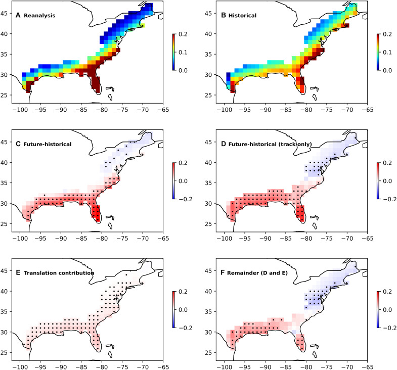
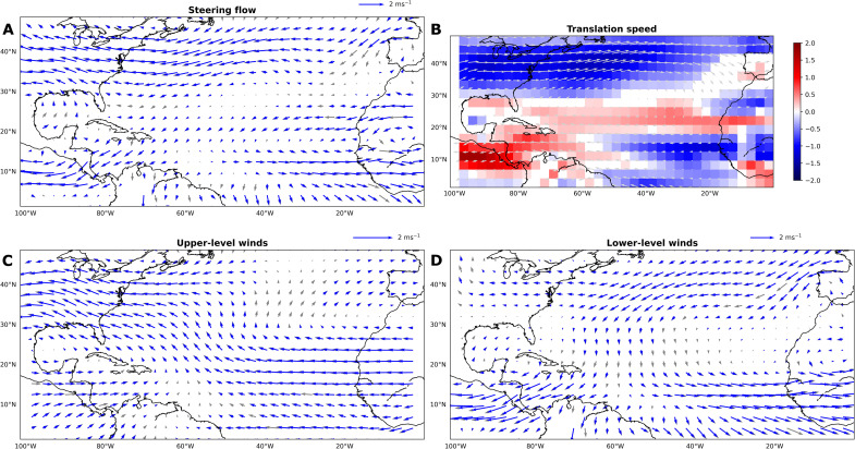
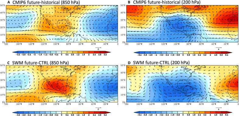
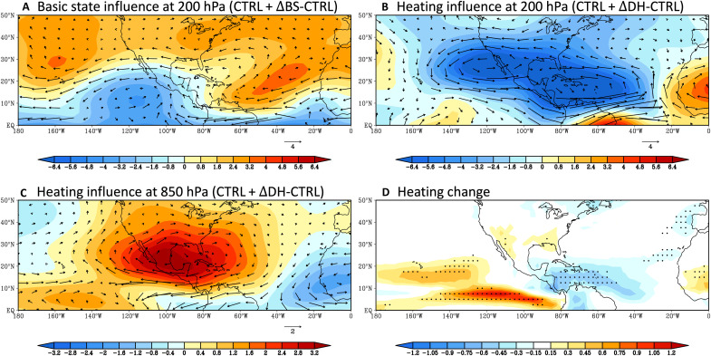
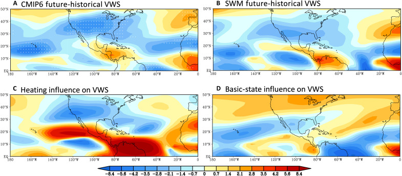
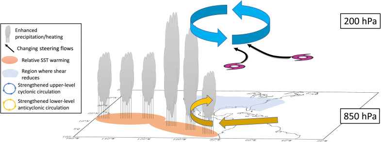
Several pathways for how climate change may influence the U.S. coastal hurricane risk have been proposed, but the physical mechanisms and possible connections between various pathways remain unclear. Here, future projections of hurricane activity (1980-2100), downscaled from multiple climate models using a synthetic hurricane model, show an enhanced hurricane frequency for the Gulf and lower East coast regions. The increase in coastal hurricane frequency is driven primarily by changes in steering flow, which can be attributed to the development of an upper-level cyclonic circulation over the western Atlantic. The latter is part of the baroclinic stationary Rossby waves forced mainly by increased diabatic heating in the eastern tropical Pacific, a robust signal across the multimodel ensemble. Last, these heating changes also play a key role in decreasing wind shear near the U.S. coast, further aggravating coastal hurricane risk enhanced by the physically connected steering flow changes.

Fig. 1.. Projected change in U.S. hurricane risk based on Risk Analysis Framework for Tropical Cyclones (RAFT).

(A) Climatological coastal hurricane frequency (CHF), defined as the number of 6-hour hurricane track locations per square degree per year, obtained when RAFT is used with reanalysis (1979–2018). All track locations where the storm intensity exceeds 25 knots are used. (B) Climatological CHF obtained when RAFT is used with historical phase 6 of the Coupled Model Intercomparison Project (CMIP6) simulations. Ensemble mean of eight models for the historical period 1980–2014 is shown. All track locations where the storm intensity exceeds 21.5 knots are used to estimate CHF. (C) Change in CHF for the future period (2066–2100) with respect to the historical period (1980–2014) under the SSP585 emissions scenario. (D) As in (C) but based only on the track model in RAFT. A 2-day cutoff is used to truncate tracks over land. (E) Change in CHF for the future period based on projected change in translation speed. (F) Contribution of projected change in landfall to future change in CHF estimated as the difference between (D) and (E). In (C) to (F), black dots indicate those locations where seven of the eight models agree on the sign of the change.

Fig. 2.. Projected changes in the environmental steering flow under the SSP585 scenario.

(A) Vector changes in steering flow. (B) Changes in translation speed (shaded) with vectors of climatological steering flow from the historical period overlaid. Vector changes in winds at (C) upper level (200 hPa) and (D) lower level (850 hPa). Note that the winds at the upper and lower levels are multiplied by 0.2 and 0.8, respectively, to reflect their relevance to the steering flow. Changes are based on the ensemble mean of eight phase 6 of the Coupled Model Intercomparison Project (CMIP6) models. All parameters are averaged over the months of August to October. “Change” indicates the difference between the mean over the future period (2066–2100) and the historical period (1980–2014). In (A), (C), and (D), blue arrows indicate locations where changes in vector magnitude are statistically significant at the 95% level based on the Student’s t test. In (B), nonwhite shaded areas represent locations where changes in translation speed are significant at the 95% level based on the Student’s t test.

Fig. 3.. Changes in the large-scale wind patterns under the SSP585 scenario simulated by the stationary wave model (SWM).

Projected changes in streamfunction (shaded, 10⁶ m²s⁻¹) and winds (vector, ms⁻¹) simulated by the ensemble mean of eight phase 6 of the Coupled Model Intercomparison Project (CMIP6) models at (A) 850 and (B) 200 hPa. In (A) and (B), white stippling denotes the areas where the changes in streamfunction are statistically significant at 95% level based on the Student’s t test. (C) and (D) are same as (A) and (B), but for changes simulated by the SWM. All parameters are averaged over the months of August to October. Change indicates the difference between the mean over the future period (2066–2100) and the historical period (1980–2014). EQ, equator.

Fig. 4.. Understanding changes in the large-scale wind patterns under the SSP585 scenario using the stationary wave model (SWM).

(A) Contribution from the anomalous zonal-mean basic state to changes in the streamfunction (shaded, 10⁶ m²s⁻¹) and winds (vector, ms⁻¹) at 200 hPa. (B) Same as (A), but for the contribution from the anomalous zonally asymmetric diabatic heating. (C) Same as (B), but at 850 hPa. (D) Projected changes in column-averaged pressure-weighted diabatic heating (K day⁻¹). Stippling indicates locations where the ensemble-mean changes are statistically significant at the 95% level. All parameters are averaged over the months of August to October. Change indicates the difference between the mean over the future period (2066–2100) and the historical period (1980–2014). EQ, equator.

Fig. 5.. Understanding changes in vertical wind shear under the SSP585 scenario.

(A) Projected changes in wind shear (ms⁻¹) by the ensemble mean of eight phase 6 of the Coupled Model Intercomparison Project (CMIP6) models. White stippling denotes the regions where the changes in wind shear are statistically significant at the 95% level. VWS, vertical wind shear. (B) is same as (A), but for changes simulated by the SWM. (C) Contribution from the anomalous diabatic heating to changes in shear. (D) Same as (C), but for contribution from the anomalous zonal-mean basic state. EQ, equator.

Fig. 6.. Schematic illustration of the main mechanisms of coastal hurricane frequency (CHF) changes identified in this study.

As the climate warms, an increase in CHF for the U.S. Gulf and lower East coasts is projected to occur and is driven primarily by changes in steering flow. The strengthening upper tropospheric cyclonic circulation above the western Atlantic plays a pivotal role in the steering flow changes. Also, the contrasting upper- and lower-level circulation anomalies reduce the vertical wind shear near the U.S. coastal regions. These changes in circulation can be regarded as a response to the projected increases in diabatic heating and warmer sea surface temperature (SST) over the eastern tropical Pacific, which is a robust signal across the phase 6 of the Coupled Model Intercomparison Project (CMIP6) multimodel ensemble.

References

1. J. Weinkle, C. Landsea, D. Collins, R. Musulin, R. P. Crompton, P. J. Klotzbach, R. Pielke, Normalized hurricane damage in the continental United States 1900–2017. Nat. Sustain. 1, 808–813 (2018).
1. P. J. Klotzbach, S. G. Bowen, R. Pielke, M. Bell, Continental U.S. hurricane landfall frequency and associated damage: Observations and future risks. Bull. Am. Meteorol. Soc. 99, 1359–1376 (2018).
1. A. Grinsted, P. Ditlevsen, J. H. Christensen, Normalized US hurricane damage estimates using area of total destruction, 1900-2018. Proc. Natl. Acad. Sci. U.S.A. 116, 23942–23946 (2019). - PMC - PubMed
1. J. S. Petterson, L. D. Stanley, E. Glazier, J. Philipp, A preliminary assessment of social and economic impacts associated with Hurricane Katrina. Am. Anthropol. 108, 643–670 (2006).
1. J. B. Halverson, T. Rabenhorst, Hurricane Sandy: The science and impacts of a superstorm. Weatherwise 66, 14–23 (2013).