[Preprint]. 2024 Sep 6:2023.03.31.535173.
doi: 10.1101/2023.03.31.535173.

Reward timescale controls the rate of behavioural and dopaminergic learning

Affiliations

Reward timescale controls the rate of behavioural and dopaminergic learning

Dennis A Burke et al. bioRxiv. .

Abstract

Learning the causes of rewards is necessary for survival. Thus, it is critical to understand the mechanisms of such a vital biological process. Cue-reward learning is controlled by mesolimbic dopamine and improves with spacing of cue-reward pairings. However, whether a mathematical rule governs such improvements in learning rate, and if so, whether a unifying mechanism captures this rule and dopamine dynamics during learning remain unknown. Here, we investigate the behavioral, algorithmic, and dopaminergic mechanisms governing cue-reward learning rate. Across a range of conditions in mice, we show a strong, mathematically proportional relationship between both behavioral and dopaminergic learning rates and the duration between rewards. Due to this relationship, removing up to 19 out of 20 cue-reward pairings over a fixed duration has no influence on overall learning. These findings are explained by a dopamine-based model of retrospective learning, thereby providing a unified account of the biological mechanisms of learning.


Figures
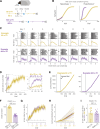
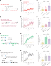
Fig. 1.
Fig. 1.. Behavioral learning in one-tenth the experiences with ten times the trial spacing.
A, Schematic of experimental setup. Head-fixed mice were divided into two groups that were each presented with identical cue-reward pairing trials, but each group differed in the duration from a reward to the next cue (i.e., the inter-trial interval or ITI). Mice were conditioned for one hour per day resulting in 50 (60 s ITI) or 6 (600 s ITI) trials per session (see Methods). B, Illustration of two hypothetical experimental outcomes. Learning curves display the possible relationship between group-averaged learning rates for 60 s and 600 s ITI as a function of trial number. C, Example lick raster plots (upper row) and lick peri-stimulus time histograms (PSTH) (lower row) for one example mouse from either 60 s ITI group (top, gold) or 600 s ITI group (bottom, purple) showing every cue and reward presentation across eight days of conditioning. Each column represents a single day of conditioning. Graphs are aligned to cue onset (cue duration denoted by gray shading). Reward delivery is denoted by the vertical gray dashed line. This convention is followed for all similar figures later in the manuscript. Both example animals begin to show evidence of learning (an increase in licking following cue onset before reward is delivered) on day 2. D, 600 s ITI mice learn and reach asymptotic behavior in fewer trials than 60 s ITI mice. Left, Timecourse showing the average change in cue-evoked lick rate (the baseline subtracted lick rate between cue onset and reward delivery, see Methods) over 40 (600 s ITI, purple, n = 19 mice) or 400 (60 s ITI, gold, n = 19 mice) cue-reward presentations. Inset right, Zoom in of first 40 trials for both groups. Lines represent mean across animals and shaded area represents the SEM. E, Cumulative sum (cumsum) of cue-evoked licks across trials from the same example mice as in C. Using the cumsum curve from each animal to determine the trial after which mice first show evidence of learning (fig. S2; see Methods), we found that the example 60 s ITI mouse (left, gold) learns after trial 74, while 600 s ITI group (right, purple) learns after trial 8 (i.e., “few shot” reward learning). Learned trial is denoted by the solid black vertical line. F, 600 s ITI mice learn in about ten times fewer trials than 60 s ITI mice. Bar height represents mean trial after which mice show evidence of learning for 60 s ITI group (left, gold, n = 17) and 600 s ITI group (right, purple, n = 19), plotted on a log scale. Error bar represents SEM. Circles represent individual mice. Values under labels represent mean ± SEM. Two mice that did not show evidence of learning are excluded from comparison (fig. S2; see Methods). **** p < 0.0001, Welch’s t-test, F-test. G - H, On average, learning between groups progresses similarly as a function of total conditioning time, and thus scales with the ratio of ITIs. G. Average cue-evoked lick rates for 600 s ITI and 60 s ITI groups across scaled trial numbers (same data as in D), showing that the 600 s ITI group learns ten times more per experience compared to the 60 s ITI group. H. Cumsum of cue-evoked licks plotted on the same scaled x-axis. Thick lines represent group means and thin lines represent individual animals. Note the higher individual variability in the 60 s ITI group compared to the 600 s ITI group (quantified in I). I, Asymptotic cue-evoked lick rates have similar group means, but different variances. Bars represent mean cue-evoked lick rates during trials 301–400 (60 s ITI) or trials 31–40 (600 s ITI). Error bars represent SEMs and circles represent individual mice. ns: not significant, Welch’s t-test; **p<0.01, F-test. See table S1 for full statistical test details from all figures including test statistics, n’s, degrees of freedom, and both corrected and uncorrected p-values.All error bars and shading throughout the manuscript represent SEM unless otherwise noted. Values displayed under bar graph labels represent mean ± SEM.
Fig. 2.
Fig. 2.. Dopaminergic learning in one-tenth the experiences with ten times the trial spacing.
A, Schematic of mesolimbic dopamine measurements from nucleus accumbens core (NAcC; see Methods). B, Diagrams of two hypothetical relationships between dopaminergic and behavioral learning in 60 s and 600 s ITI mice. C, Example lick raster plots (upper row), lick PSTH (2nd row), heatmap of dopamine responses on each trial (3rd row) and average dopamine PSTH for the day (lower row) for one example mouse from either 60 s ITI group (top, gold) or 600 s ITI group (bottom, purple) showing every cue and reward presentation across eight days of conditioning. Lick data presented as in Fig. 1C. Dopamine signals plotted as % dF/F. Graphs aligned to cue onset (cue duration denoted by gray shading). Reward delivery is denoted by vertical gray dashed line. D, Cumsum of cue-evoked licks (solid, left axis) or of cue-evoked dopamine (dashed, right axis) for the same example mice as in C. Both lick and cue-evoked dopamine values were divided by total trial number to display average responses across conditioning. Before taking the cumsum, cue-evoked dopamine responses were normalized by max reward responses for each animal (see Methods). Cumsum curves were used to determine the trial after which cue-evoked dopamine or cue-evoked licking emerge (“learned trial”, see Methods). Solid vertical lines represent learned behavior trial and dashed vertical lines represent dopamine learned trial. This convention is followed for all similar figures later in the manuscript. E, Dopamine responses to cue develop in ten times fewer trials in 600 s ITI mice compared to 60 s ITI mice. Values under labels represent mean ±SEM across mice. * p<0.05, Welch’s t-test. F, On average, DA cue responses develop 60 trials before the emergence of cue-evoked licking in 60 s ITI mice and 5 trials before in 600 s ITI mice. **p<0.01. Welch’s t-test. G, Average cumsum of cue-evoked licks (solid) and dopamine (dashed) across groups. Data were normalized by each animal’s final trial of conditioning and aligned to their learned trial before averaging. Lines represent means, and shading represents SEM. H, Average cumsum of normalized cue-evoked dopamine responses in 60 s ITI (gold) and 600 s ITI (purple) mice. Cumsum curves divided by number of trials to account for differences between groups. I, Mean asymptotic normalized cue-evoked dopamine after learning. Bars represent means for trials 301–400 (60 s ITI) or trials 31–40 (600 s ITI). Error bars represent SEM and circles represent individual mice. *p<0.05, Welch’s t-test.
Fig. 3.
Fig. 3.. Learning rate scales proportionally with reward frequency across a range of trial spacing intervals.
A, 30 s ITI and 300 s ITI conditioning (total number of trials a day 30 s: 100, 300 s: 11). B, Example lick raster plots (upper row) and lick PSTH (lower row) for one example mouse from either 30 s ITI (top, orange) or 300 s ITI groups (bottom, pink) showing every cue and reward presentation across eight days of conditioning. Data presented as in Fig. 1C. C, Cumsum of cue-evoked licks across trials from the same example mice as in B. Learned trial is denoted by the solid black vertical line. D, 300 s ITI mice learn and reach asymptotic behavior in fewer trials than 30 s ITI mice. Timecourse showing the average change in cue-evoked lick rate over 80 (300 s ITI, pink, n = 6) or 800 (30 s ITI, orange, n = 6) cue-reward presentations. E, 300 s ITI mice learn in about ten times fewer trials than 30 s ITI mice. One mouse that did not show evidence of learning is excluded from comparison (fig. S5C; see Methods). * p < 0.05, Welch’s t-test. F, Cumsum of cue-evoked licks (i.e., of data in D) plotted across scaled trials. G, Average cue-evoked lick rates for 30 s (orange, same data as D), 60 s (gold, same data as Fig. 1, D and G), 300 s (pink, same data as D), and 600 s (purple, same data as Fig. 1, D and G) across scaled trial numbers. On average, learning between groups scales with the ratio of ITIs and progresses similarly as a function of total conditioning time. Lines represent mean across animals and shaded area represents the SEM. H, Mean trials to learn for different ITI groups as a function of inter-reward interval (IRI) plotted on a log-log axis. Circles represent mean trials to learn per group and error bars represent standard deviation. Solid black line is best fit regression line (R2 = 0.9992, *** p<0.001). Slope is not significantly different from −1 (one-sample t-test) indicating a proportional quantitative scaling relationship between IRI and learning rate (1/trials to learn). I, A group of animals with a 3600 s ITI were conditioned similarly to previous groups to test if the observed power law relationship between IRI and trials to learn holds at extreme IRIs. Animals were presented with two cue-reward pairings per session for a total session duration of 2 hours. J, Example lick raster plots (upper row), lick PSTH (2nd row), heatmap of dopamine responses on each trial (3rd row) and dopamine PSTH (lower row) for one example 3600 s ITI mouse showing every cue and reward presentation across eight days of conditioning. Data presented as in Fig. 2C. K, Cumsum of cue-evoked licks (solid, left axis) or of normalized cue-evoked dopamine (dashed, right axis) for the same example mouse as in J. Data presented as in Fig. 2D. L, Average cumsums of cue-evoked licks and normalized cue-evoked dopamine in 3600 s ITI mice (n = 5). M, Number of trials for 3600 s ITI (n = 5) mice to learn cue-reward association. Bar height represents mean trial after which mice show evidence of learning. Dashed line represents predicted trials to learn based on relationship observed for 30 s – 600 s ITI groups (best fit line in H). Values under labels represent mean ± SEM. *** p< 0.001, one-sample t-test. N, 3600 s ITI mice (blue circle, filled) take more trials to learn than predicted from the proportional scaling relationship in H. White filled circles and line are same data as H. Dashed lines represent predicted and mean observed trials to learn for 3600 s ITI. O, Learning in 3600 s ITI mice does not scale proportionally with other groups. Average cue-evoked lick rates for 30 s, 60 s, 300 s, 600 s, (30–600 s ITI, same data as G) and 3600 s ITI (blue, n = 5) mice across scaled trial numbers. Previously displayed data are shown without error to aid visualization. P, Mean dopamine learned trial for 3600 s ITI mice (n = 5). Values under labels represent mean ± SEM. Q, Average cumsum of normalized cue-evoked dopamine responses in 60 s ITI (gold, same data as Fig. 2H), 600 s ITI (purple, same data as Fig. 2H), and 3600 s ITI (blue, n = 5) mice. Cumsum curves divided by number of trials to account for differences between groups. Transparency added to previously displayed data to aid visualization. Shaded region represents SEM. R, Asymptotic normalized cue-evoked dopamine after learning is highest in 3600 s ITI mice. Bars represent means for trials 301–400 (60 s ITI, same data as Fig. 2I), trials 31–40 (600 s ITI, same data as Fig. 2I), or trials 15–16 (3600 s ITI mice). Transparency added to previously displayed data to aid visualization. *p<0.05, Welch’s t-test.
Fig. 4.
Fig. 4.. Proportional scaling of learning rate by inter-reward interval is only captured by a retrospective learning model.
A, Diagram of number of trials experienced by each ITI group over a ten-minute interval. Based on the experimentally observed proportional scaling between trial spacing and learning rate (Fig. 3H), learning is equivalent during this interval regardless of the number of trials experienced for 30 s – 600 s ITI, but not 3600 s ITI mice. Note that multiple 3600 s trials are not shown to maintain the scale of the diagram. B, Total conditioning time prior to the emergence of anticipatory licking from experiments in Figs. 1 and 3. Symbols represent individual mice, and bar height represents mean across ITI group. C, Schematic diagram of microstimulus implementation of temporal difference reinforcement learning (TDRL). At each moment, a value estimate of future rewards is updated by a reward prediction error (RPE), representing a deviation from current value estimate that is thought to be encoded in the brain by dopamine signaling. Value is used to drive behavioral responding. The microstimulus implementation of TDRL was specifically chosen because external stimuli (i.e. cues and rewards) evoke microstimuli which spread representations of the external stimuli in time. Because the model contains ITI states that themselves can acquire value, the model contains a potential mechanism to explain how the spacing between trials could affect learning rate. Parameter combinations were swept to determine if any set could capture the quantitative scaling observed in the experimental results where learning rate varied proportionally with the IRI. D, Trials to learn (when value > threshold) as a function of IRI for TDRL simulation with parameter combination that best fits experimental results (see Methods). Hexagons represent mean trials to learn across iterations (n = 20 each) for all conditions. Open circles represent experimental data (same as Fig. 3, H and N). Akaike information criterion (AIC) model weight comes from comparison with best fit SOP (F), and ANCCR (I) models. Please note that this AIC model does not penalize free parameters, i.e., is a conservative estimate biased against ANCCR (see Methods for rationale and table S1 for AIC model weight when penalizing for parameters). E, Timecourse of value on each trial (maximum between cue and reward) for best fit TDRL model (B) averaged across iterations (n = 20 each) and plotted across scaled trials for all conditions. SEM occluded by thickness of mean lines. F, Total conditioning time prior to the emergence of behavior (threshold crossing). Symbols represent time for a single iteration, and bar height represents mean (n = 20 iterations per ITI condition). G, Schematic diagram of Wagner’s SOP (Standard Operating Procedure or Sometimes Opponent Process) model of associative learning. Presentations of cues or rewards evoke presumed mental representations or processing nodes consisting of many informational elements. These stimulus representations are dynamic: presentation of a stimulus moves a portion of elements from (only) the inactive (I) state into the primary active state (A1). Elements then decay into the secondary active state (A2) and then decay again back to the inactive state while the stimulus is absent. Elements transition between states according to individually specified probabilities. Cue-reward associations (value) are strengthened and learned when cue elements in A1cue and reward elements in A1reward overlap in time. Following learning, cues evoke conditioned responding by directly activating reward elements to their A2 state. One way in which SOP has been hypothesized to explain ITI impact on learning is that more time between trials allows more elements to decay to the inactive state, allowing for greater number of elements to transition to the A1 active state upon next cue and reward presentation. Parameter combinations were swept through to determine if any set of parameters could capture the quantitative scaling observed in the experimental results. H, Trials to learn (when value > threshold) as a function of IRI for SOP simulation with best-fit parameter combination of experimental results (see Methods). Squares represent mean trials to learn across iterations (n = 20 each) for all conditions. Open circles represent experimental data (same as Fig. 3, H and N). Akaike information criterion (AIC) model weight comes from comparison with best fit TDRL (B) and ANCCR (I) models. Please note that this AIC model does not penalize free parameters, i.e., is a conservative estimate biased against ANCCR (see Methods for rationale and table S1 for AIC model weight when penalizing for parameters). I, Timecourse of value on each trial (maximum between cue and reward) for best fit SOP model (F) averaged across iterations (n = 20 each) and plotted across scaled trials. SEM occluded by thickness of mean lines. J, Total conditioning time prior to the emergence of behavior (threshold crossing). Symbols represent time for a single iteration, and bar height represents mean (n = 20 iterations per ITI condition). K, Schematic diagram of ANCCR. See text for explanation of learning rate scaling in ANCCR. L, Trials to learn (when NCcuereward (net contingency) > threshold) as a function of IRI for ANCCR simulation with parameter combination that best fits experimental results (see Methods). Crosses represent mean trials to learn across iterations (n = 20 each). Open circles represent experimental data (same as Fig. 3, H and N). Akaike information criterion (AIC) model weight comes from comparison with best fit TDRL (B) and SOP (F) models. M, Timecourse of NCcuereward on each trial for best fit ANCCR model (I) averaged across iterations (n = 20 each) and plotted across scaled trial units. SEM occluded by thickness of mean lines. N, Total conditioning time prior to the emergence of behavior (threshold crossing). Symbols represent time for a single iteration, and bar height represents mean (n = 20 iterations per ITI condition).
Fig. 5.
Fig. 5.. Learning rate scaling is not explained by number of experiences per day, context extinction, overall rate of auditory cues, or overall rate of rewards.
A - C, Number of trials per day does not explain difference in learning rates between 60 s and 600 s ITI mice. A Schematic of conditioning for ‘60 s ITI-few’ group, which were conditioned with the same ITI as 60 s ITI mice (mean: 60 s) and the same number of trials/rewards per day as 600 s ITI mice (six). B Timecourse of average cue-evoked lick rate for 60 s ITI-few (red, n = 18), 60 s ITI (same data as Fig. 1D), and 600 s ITI (same data as Fig. 1D) mice over 40 trials of conditioning. 60 s and 600 s ITI timecourses are shown transparent and without error for visualization purposes. C Mean cue-evoked lick rate between trials 36 and 40 across all three groups. 60 s ITI-few mice show significantly less cue-evoked licking than 600 s ITI mice and behave like 60 s ITI mice. ****p<0.0001, ns: not significant; Welch’s t-tests. D - F, Context extinction does not explain difference in learning rates between 60 s and 600 s ITI mice. D Schematic of conditioning for “60 s ITI-few with context extinction” group. Mice were conditioned similarly to 60 s ITI-few mice but remained in the experimental context for ~55 minutes following the end of conditioning trials, matching 600 s ITI group’s time in context and number of cue-reward experiences, while the rate of rewards during trials matched the 60 s ITI group. E Timecourse of average cue-evoked lick rate for 60 s ITI-few with context extinction (light pink, n = 6), 60 s ITI (same data as Fig. 1D), and 600 s ITI (same data as Fig. 1D) mice over 40 trials of conditioning. F Mean cue-evoked lick rate between trials 36 and 40 across all three groups. 60 s ITI-few with context extinction mice show significantly less cue-evoked licking than 600 s ITI mice and are not significantly different from 60 s ITI mice. **p<0.01, ns: not significant; Welch’s t-tests. G - I, Overall rate of auditory cues does not explain difference in learning rates between 60 s and 600 s ITI mice. G Schematic of conditioning for “60 s ITI with CS-“ group. Mice were conditioned similarly to 600 s ITI mice but during the (~600 s) interval between CS+reward trials, distractor CS- cues (3kHz pure tone) were presented on average every 60 s to match the rate of auditory cues experienced by 60 s ITI mice. All mice could hear and respond to CS- as evidenced by some amount of generalized licking observed during conditioning (fig. S10, C and D). H Timecourse of average cue-evoked lick rate for 60 s ITI with CS- (green, n = 6), 60 s ITI (same data as Fig. 1D), and 600 s ITI (same data as Fig. 1D) mice over 40 trials of conditioning. I Average cue-evoked lick rate between trials 36 and 40 across all three groups. 60 s ITI with CS- mice show significantly more cue-evoked licking compared to 60 s ITI and are not significantly different from 600 s ITI mice. ***p<0.01, ns: not significant; Welch’s t-tests. J - L. Learning rate is not scaled by overall rate of rewards. J Schematic of conditioning for “600 s ITI with background chocolate milk” group. Mice were conditioned similarly to 600 s ITI mice but during the (~600 s) interval between cuesucrose trials, mice received 2 un-cued deliveries of chocolate milk ~180 s apart to test whether cue-sucrose learning rate is affected by the general or identity specific rate of rewards. Mice readily consumed chocolate milk rewards upon delivery (fig. S10H). K Timecourse of average cue-evoked lick rate for 600 s ITI with background chocolate milk (gray, n = 6), 60 s ITI (same data as Fig. 1D), and 600 s ITI (same data as Fig. 1D) mice over 40 trials of conditioning. L Average cue-evoked lick rate between trials 36 and 40 across all three groups. 600 s ITI with background chocolate milk mice show significantly more cue-evoked licking compared to 60 s ITI and are not significantly different from 600 s ITI mice. ***p<0.01, ns: not significant; Welch’s t-tests.
Fig. 6.
Fig. 6.. Partial reinforcement scales learning rate by increasing the inter-reward interval.
A, Schematic of 60 s ITI-50% partial reinforcement conditioning. Mice were conditioned identically to 60 s ITI mice (Fig. 1) except rewards were delivered with 50% reward probability for 50 trials with ~25 rewards a day. Reducing the reward probability by 50% leads to a doubling of the IRI to ~120 s on average across a session while maintaining the ITI and ICI. Mice were conditioned for 12 days. B, Cumsum of cue-evoked licks (solid, left axis) or normalized cue-evoked dopamine (dashed, right axis) as a function of rewarded trials for all 60 s ITI-50% mice. Data presented as in Fig. 2D. Dopamine was not recorded from two initial mice and two other mice did not show evidence of behavioral learning (see Methods). C, 60 s ITI-50% mice (magenta, n = 8) learn the cue-reward association in about half the number of rewards as 60 s ITI mice (same data as Fig. 1F). Bar height represents mean number of rewards after which mice show evidence of learning.. Values under labels represent mean ± SEM. Mice that did not show evidence of learning (B) were excluded from analysis. **** p<0.0001, Welch’s t-test. D-E, Among mice that learned the cue-reward association, 60 s ITI-50% mice show lower asymptotic lick rates than 60 s ITI mice, consistent with prior literature on partial reinforcement; however, asymptotic dopamine responses do not show statistically significant difference between groups suggesting a dissociation between behavior and dopamine. Left, Timecourse of cue-evoked lick rate (D) or normalized cue-evoked dopamine (E) across all conditioning trials for 60 s ITI-50% (magenta, n = 8 behavior, n = 6 dopamine) and 60 s ITI (gold, n = 17 behavior, 5 dopamine) mice. Right, Mean cue-evoked lick rate (D) and normalized cue-evoked dopamine (E) during the last 100 trials of conditioning for both groups. **p<0.01, ns: not significant, Welch’s t-test F, Further suggesting a dissociation between behavior and dopamine, non-learner mice (red, n = 2) show intact dopaminergic learning similar to behavioral learner mice (black, n = 6). Cumsum of cue-evoked licks (left axis, solid lines) or normalized cue-evoked dopamine (right axis, dashed lines) over all 600 trials. G, Diagrams of two possible relationships between the onset of cue-evoked dopamine and the emergence of reward omission driven dopamine dips over the course of learning. H, Lick raster and heatmap of dopamine aligned to cue onset for one example 60 s ITI-50% mouse during omission (left) and rewarded (right) trials across conditioning. I, Lick (left) and dopamine (right) PSTHs aligned to cue onset for the same example mouse as in H. Light blue represents data from trials where rewards were delivered, while dark blue represents trials where rewards were omitted. Data are binned into early conditioning (trials 1–30, top), middle conditioning (trials 61–90, middle), and late conditioning (trials 261–290, bottom). In the middle row, note the prominent cue-evoked dopamine and licking and the absence of a dopamine dip following reward omission. J, On average, reward omission driven dopamine dips emerge later than cue-evoked dopamine in 60 s ITI-50% mice (n = 6). Average cumsum of normalized dopamine responses to cue presentation (green, dashed) or reward omission (magenta, dashdot) across reward omission trials. K, Omission dips emerge later than cue-evoked dopamine in individual mice. Cumsum of normalized dopamine responses to cue presentation (green, dashed) or reward omission (magenta, dashdot) across omission trials for all 60 s ITI-50% mice with dopamine recordings that learned the cue-reward association. Dashed lines on upper half of plots represent the omission trial after which cue-evoked dopamine emerges (dopamine learned trial), and dashdot lines on bottom of plot represent the omission trial after which dips in dopamine following reward omission emerge. L, On average, cue-evoked dopamine emerges 82 omission trials before dips in dopamine following reward omission. Bar height represents mean number of omissions before cue-evoked dopamine (green) or reward omission driven dips in dopamine (magenta) begin. Error bar represents SEM. Circles represent individual mice, and lines connect data from a single mouse. ** p <0.01, paired t-test.

Similar articles

References

    1. Ebbinghaus Hermann. Memory: A contribution to experimental psychology. Memory: A contribution to experimental psychology. Teachers College Press, New York, NY, US, 1913. doi: 10.1037/10011-000. - DOI
    1. Hintzman Douglas L.. Theoretical Implications of the Spacing Effect. Routledge, 1974. ISBN 978–1-03–272237-5.
    1. Cepeda Nicholas J., Pashler Harold, Vul Edward, Wixted John T., and Rohrer Doug.Distributed practice in verbal recall tasks: A review and quantitative synthesis. Psychological Bulletin, 132(3):354–380, 2006. ISSN 1939–1455. doi: 10.1037/0033-2909.132.3.354. - DOI - PubMed
    1. Cepeda Nicholas J., Vul Edward, Rohrer Doug, Wixted John T., and Pashler Harold. Spacing effects in learning: A temporal ridgeline of optimal retention. Psychological Science, 19(11): 1095–1102, November 2008. ISSN 0956–7976. doi: 10.1111/j.1467-9280.2008.02209.x. - DOI - PubMed
    1. Dempster Frank N.. Spacing effects and their implications for theory and practice. Educational Psychology Review, 1(4):309–330, December 1989. ISSN 1573–336X. doi: 10.1007/BF01320097. - DOI

Publication types