Accurate and Fast Deep Learning Dose Prediction for a Preclinical Microbeam Radiation Therapy Study Using Low-Statistics Monte Carlo Simulations

Abstract

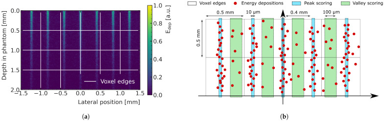
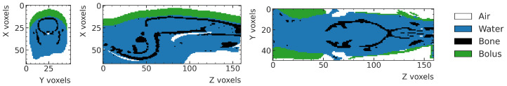
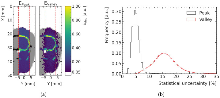
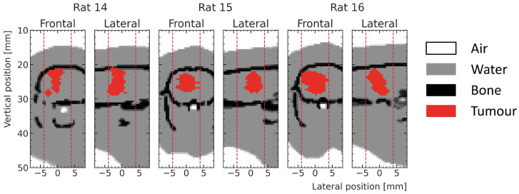
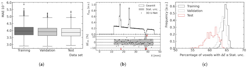
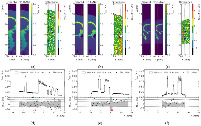
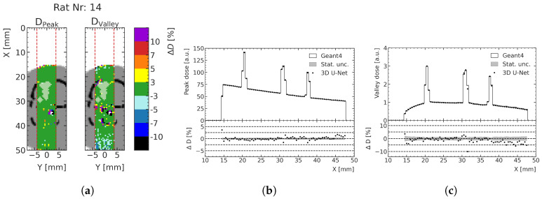
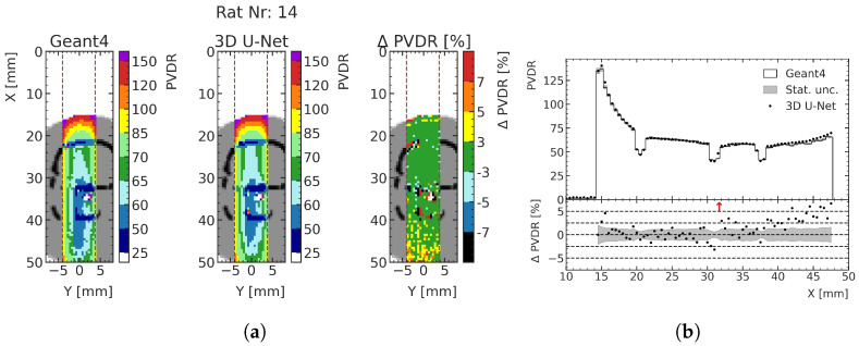
Microbeam radiation therapy (MRT) utilizes coplanar synchrotron radiation beamlets and is a proposed treatment approach for several tumor diagnoses that currently have poor clinical treatment outcomes, such as gliosarcomas. Monte Carlo (MC) simulations are one of the most used methods at the Imaging and Medical Beamline, Australian Synchrotron to calculate the dose in MRT preclinical studies. The steep dose gradients associated with the 50μm-wide coplanar beamlets present a significant challenge for precise MC simulation of the dose deposition of an MRT irradiation treatment field in a short time frame. The long computation times inhibit the ability to perform dose optimization in treatment planning or apply online image-adaptive radiotherapy techniques to MRT. Much research has been conducted on fast dose estimation methods for clinically available treatments. However, such methods, including GPU Monte Carlo implementations and machine learning (ML) models, are unavailable for novel and emerging cancer radiotherapy options such as MRT. In this work, the successful application of a fast and accurate ML dose prediction model for a preclinical MRT rodent study is presented for the first time. The ML model predicts the peak doses in the path of the microbeams and the valley doses between them, delivered to the tumor target in rat patients. A CT imaging dataset is used to generate digital phantoms for each patient. Augmented variations of the digital phantoms are used to simulate with Geant4 the energy depositions of an MRT beam inside the phantoms with 15% (high-noise) and 2% (low-noise) statistical uncertainty. The high-noise MC simulation data are used to train the ML model to predict the energy depositions in the digital phantoms. The low-noise MC simulations data are used to test the predictive power of the ML model. The predictions of the ML model show an agreement within 3% with low-noise MC simulations for at least 77.6% of all predicted voxels (at least 95.9% of voxels containing tumor) in the case of the valley dose prediction and for at least 93.9% of all predicted voxels (100.0% of voxels containing tumor) in the case of the peak dose prediction. The successful use of high-noise MC simulations for the training, which are much faster to produce, accelerates the production of the training data of the ML model and encourages transfer of the ML model to different treatment modalities for other future applications in novel radiation cancer therapies.

Keywords: Geant4; Monte Carlo simulation; deep learning; dose prediction; microbeam radiation therapy; preclinical study.

Figure 1

(a) Energy deposition in water by a subset of coplanar X-ray microbeams, typical of MRT, entering from the top of the shown region. The dose is deposited mainly along the tracks of the X-rays (peaks regions). The peaks are separated by valleys where the dose is significantly lower. Macrovoxels are shown in white. (b) Sketch showing the concept of scoring energy deposition into macrovoxels (represented as white pixels with 0.5 mm lateral sizes). The energy deposition is calculated in the peaks (light blue regions) and in the valleys (green regions) and then associated to the macrovoxel containing it. Adapted from [23].

Figure 2

Example of digital rat phantom obtained from the segmentation of CT scans. Defined materials (air, water and bone) are assigned to individual voxels. Green voxels are associated to the bolus, modeled as water.

Figure 3

(a) Two-dimensional slice of the MC-simulated energy deposition in the peak (left) and valley (right), respectively, at the center of the prediction volume for an exemplary high-noise training sample (rat number 1), normalized to their respective maximum. The prediction volume is indicated with red dashed lines. Air is shown white, tissue (water) in gray and bone in black. (b) Histograms of the voxelwise statistical uncertainties (quantified with the standard error) of the peak and valley energy deposition MC simulations in the high-noise datasets.

Figure 4

Frontal and lateral slices at the center of the ML prediction regions (red dotted lines) showing exemplary tumors (red) in the respective phantoms (white—air, gray—water and black—bone) of the three test rats used in the testing.

Figure 5

(a) Two-dimensional slice of the MC-simulated energy deposition in the peak (left) and valley (right), respectively, at the center of the prediction volume for an exemplary low-noise training sample (rat number 15), normalized to their respective maximums. Air is shown in white, tissue (water) in gray and bone in black. (b) Histograms of the voxelwise statistical uncertainties (quantified with the standard error) of the peak and valley energy deposition MC simulations of the three low-noise treatment test data samples.

Figure 6

Schematic of the implemented deep learning model predicting energy deposition based on a material matrix input. Adapted from [22].

Figure 7

Overview of the validation loss values (diamonds) and the corresponding training data loss values (open circles) for different valley (a) and peak (b) energy deposition prediction model configurations. The x-ticks locate the different investigated learning rates, while the batch sizes and number of filters are highlighted for each model by their positioning in the respective white (batch size) and colored (number of filters) boxes. The best respective model is marked with a red circle.

Figure 8

(a) Boxplots showing the MAE in the valley region for the training, validation and test datasets. The central line of the each boxplot shows the median of the distribution. The surrounding box is limited by the 25% percentile. The whiskers are shown at the 2.5 × 25% percentile. Data samples further away from the median are represented as outliers. (b) Exemplary ML-predicted and MC-simulated energy deposition $E_{\mathrm{dep}}$ of the validation data in the valley region. The bottom plot shows the percent relative difference $\Delta E_{\mathrm{rel}}$ between ML prediction and MC simulation in terms of energy deposition. Red arrows in the relative energy deviation subplot indicate deviations larger than the shown ranges. (c) Fraction of voxels of the ML-predicted energy deposition maps exhibiting a deviation of one standard deviation or less with respect to the mean energy deposition $\Delta E$ calculated with the MC simulation.

Figure 9

(a) Boxplots showing the MAE in the peak region for the training, validation and test datasets. The central line of the each boxplot shows the median of the distribution. The surrounding box is limited by the 25% percentile. The whiskers are shown at the 2.5 × 25% percentile. Data samples further away from the median are represented as outliers. (b) Exemplary ML-predicted and MC-simulated energy deposition $E_{\mathrm{dep}}$ of the validation data in the peak region. The bottom plot shows the percent relative difference $\Delta E_{\mathrm{rel}}$ between ML prediction and MC simulation in terms of energy deposition. Red arrows in the relative energy deviation subplot indicate deviations larger than the shown ranges. (c) Fraction of voxels of the ML-predicted energy deposition maps exhibiting a deviation of one standard deviation or less with respect to the mean energy deposition $\Delta E$ calculated with the MC simulation.

Figure 10

(a) Exemplary peak prediction of a training data sample including a larger proportion of spine, showing a 2D slice of MC simulation and ML prediction with the difference in units of statistical standard deviations. (b,c) show two worst-case prediction cases following different criteria. (b) Test data sample with the largest average deviation between ML and MC in units of standard deviations in the peak region. (c) Test data sample with the lowest fraction of voxels in which ML prediction with MC simulation agree within one standard deviation in the valley. (d–f) The depth–energy deposition curve at the position indicated with red (black) dashed line for each 2D representation shown in (a–c). Red arrows in the relative energy deviation subplot below indicate deviations larger than the shown ranges.

Figure 11

(a) Relative dose difference ($\Delta D_{rel}$) between ML and MC models for test rat number 14 in the peak and valley regions. The tumor volume in the shown slice is indicated with a white overlay: (b) depth–peak dose curves; (c) depth–valley dose curve at the center of the prediction volume. Doses are normalized to the valley doses at the center of the brain.

Figure 12

Exemplary comparison of PVDR computed from MC simulation and ML prediction. (a) $\Delta$ PVDR is calculated as $(PVD{R}_{ML}-PVD{R}_{MC})/PVD{R}_{ML}$ for each macrovoxel (see Section 2.2). (b) Red arrows in the relative PVDR deviation subplot indicate deviations larger than the shown ranges.

References

1. Schiavi A., Senzacqua M., Pioli S., Mairani A., Magro G., Molinelli S., Ciocca M., Battistoni G., Patera V. Fred: A GPU-accelerated fast-Monte Carlo code for rapid treatment plan recalculation in ion beam therapy. Phys. Med. Biol. 2017;62:7482–7504. doi: 10.1088/1361-6560/aa8134. - DOI - PubMed
1. Kontaxis C., Bol G.H., Lagendijk J.J., Raaymakers B.W. DeepDose: Towards a fast dose calculation engine for radiation therapy using deep learning. Phys. Med. Biol. 2020;65:075013. doi: 10.1088/1361-6560/ab7630. - DOI - PubMed
1. Pastor-Serrano O., Perkó Z. Learning the Physics of Particle Transport via Transformers. arXiv. 2021 doi: 10.1609/aaai.v36i11.21466.2109.03951 - DOI
1. Jensen P.J., Zhang J., Koontz B.F., Wu Q.J. A Novel Machine Learning Model for Dose Prediction in Prostate Volumetric Modulated Arc Therapy Using Output Initialization and Optimization Priorities. Front. Artif. Intell. 2021;4:41. doi: 10.3389/frai.2021.624038. - DOI - PMC - PubMed
1. Mentzel F., Kröninger K., Lerch M., Nackenhorst O., Rosenfeld A., Tsoi A.C., Weingarten J., Hagenbuchner M., Guatelli S. Small beams, fast predictions A comparison of machine learning dose prediction models for proton minibeam therapy. Med. Phys. 2022 doi: 10.1002/mp.16066. - DOI - PubMed
LinkOut - more resources