The stability of transient relationships

Abstract

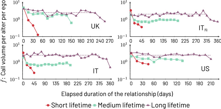
In contrast to long-term relationships, far less is known about the temporal evolution of transient relationships, although these constitute a substantial fraction of people's communication networks. Previous literature suggests that ratings of relationship emotional intensity decay gradually until the relationship ends. Using mobile phone data from three countries (US, UK, and Italy), we demonstrate that the volume of communication between ego and its transient alters does not display such a systematic decay, instead showing a lack of any dominant trends. This means that the communication volume of egos to groups of similar transient alters is stable. We show that alters with longer lifetimes in ego's network receive more calls, with the lifetime of the relationship being predictable from call volume within the first few weeks of first contact. This is observed across all three countries, which include samples of egos at different life stages. The relation between early call volume and lifetime is consistent with the suggestion that individuals initially engage with a new alter so as to evaluate their potential as a tie in terms of homophily.

Figure 1

Average per alter per ego phone call volume $\overline{f}(a,\ell )$ as a function of elapsed relationship duration a, binned with $\mathrm{\Delta }a=15$ and $\mathrm{\Delta }\ell =50$ for the four cohorts shown. The lifetime groups correspond to $\ell =0$ (short), $\ell =\lfloor ({\mathcal{L}}_{\mathcal{E}}-\mathrm{\Delta }\ell )/2\rfloor$ (medium), and $\ell ={\mathcal{L}}_{\mathcal{E}}-\mathrm{\Delta }\ell$ (long). To calculate the exact $\ell$ per country, as stated in Fig. S1 of the Supplementary Information, we use ${\mathcal{L}}_{\text{UK}}=270$; ${\mathcal{L}}_{{\text{IT}}_n}=365$; ${\mathcal{L}}_{\text{IT}}=365$; and ${\mathcal{L}}_{\text{US}}=220$. The transient condition is $\mathrm{\Delta }{t}_w=60$ days, and for cohort IT${}_n$, the gap between the entry of an ego and the acceptance of an ego-alter pair is set to $\mathrm{\Delta }{t}_s=50$ days. The number of resulting ego-alter pairs induced by our selection criteria is reported in Table 2. Robustness checks with different values for parameters $\mathrm{\Delta }\ell ,\mathrm{\Delta }a,\mathrm{\Delta }{t}_w$, and $\mathrm{\Delta }{t}_s$ are shown in the Supplementary Information, Sect. S3. The curves are stable for medium and long lifetime groups. For curves displaying stable regions, we show a dashed line that represents $b(\ell )$, the average number of phone calls to alters of a given $\ell$ during the stable regime of communication.

Figure 2

$b(\ell )$ as a function of $\ell$ obtained through the stable region average method (see Methods section). The vertical axis is in logarithmic scale. Clearly, $b(\ell )$ has an increasing trend with respect to $\ell$, with minor exceptions. The UK and US cohorts display a faster increase than IT and IT${}_n$. This could be a consequence of specific differences between details of the cohort participants, such as country, age, and/or personal circumstances of the participants; for example, since the Italian cohort is focused on adult parents with pre-teenage children, these participants may have less available time to invest in phone communication.

Figure 3

Panel (A): Box plots for all cohorts using the 1.5 interquartile range convention for p-values from Kolmogorov-Smirnov tests for egos in medium (teal) and long (purple) lifetimes in all cohorts. The per alter call averages ${\overline{f}}_i(a,\ell )$ are divided into two equally-sized ranges of a, the early range $\mathrm{\Delta }a\le a<\lfloor (1/2)\left(\lfloor ,\ell ,/,\mathrm{\Delta },a,\rfloor ,-,1\right)\rfloor \mathrm{\Delta }a$ and the late range $\lfloor (1/2)\left(\lfloor ,\ell ,/,\mathrm{\Delta },a,\rfloor ,-,1\right)\rfloor \mathrm{\Delta }a\le a\le \lfloor \ell /\mathrm{\Delta }a\rfloor \mathrm{\Delta }a-\mathrm{\Delta }a$). Large p-values mean that the early and late ranges of ${\overline{f}}_i(a,\ell )$ are not distinguishable, and thus, show no trend with a; small p-values mean there is a trend in a. We draw a dashed line at the 0.05 significance threshold and the averages over all egos are represented with the symbol $\times$. As it is clear from the plot, the vast majority of egos show no trend with a. Panel (B): Average values of $b_i(\ell )$ (circles) and standard error of the means (whiskers) for medium (teal) and long (purple) lifetimes for all cohorts. Superimposed to each circle and associated whisker is a symbol $\times$ that represents the value of $b(\ell )$ for the corresponding cohort, which matches well the averages of $b_i(\ell )$ across cohorts and lifetimes.

Figure 4

Survival probability $P(a\mid a_o,a_f,\gamma )$ of transient alters to duration of at least a for different bins $\gamma$ of amount of mobile phone calls between $a_o=30$ and $a_f=60$ days. We use the combined data for UK, Italy and US, and therefore, we only look at relationships active for $\ell <{\mathcal{L}}_{\text{US}}=220$ days or less, in order to include data for all three cohorts. The bins represented by $\gamma$ as the exponent in $3^{\gamma }\le g<3^{\gamma +1}$ are $\gamma =0,1,2,3$. As $\gamma$ increases, the probability of survival also increases, i.e. for ${\gamma }^{\prime }>\gamma$, $P(a\mid a_o,a_f,{\gamma }^{\prime })>P(a\mid a_o,a_f,\gamma )$ which is equivalent to saying that $P(a\mid a_o,a_f,\gamma )$ decays more slowly in terms of a as $\gamma$ increases. See Supplementary Information, Fig. S19, for various combinations of $a_o,a_f$.

Figure 5

Comparison between the survival probabilities $P(a\mid a_o,a_f,\gamma )$ for the combined UK and US data sets (color map) and the Italian data set (symbols). The different colors of the background represent ranges of $P_{\mathrm{UK}+\mathrm{US}}(a\mid a_o,a_f,\gamma )$, namely [0, 0.25) (red), [0.25, 0.5) (teal), [0.5, 0.75) (purple), and [0.75, 1] (yellow). Panel (A) shows the symbol $\blacksquare$ for $P_{\text{IT}}(a\mid a_o,a_f,\gamma )$ in the interval [0, 0.25), panel (B) shows the symbol $\diamond$ for the interval [0.25, 0.5), panel (C) uses the symbol $\bullet$ for the interval [0.5, 0.75), and panel (D) uses the symbol $▴$ for the interval [0.75, 1). The match in location between the symbols and the colored regions means that the behavior of different cohorts is consistent, supporting the reliability of g as a helpful predictor of $\ell$.

References

1. Holt-Lunstad J, Smith TB, Layton JB. Social relationships and mortality risk: A meta-analytic review. PLoS Med. 2010;7:e1000316. doi: 10.1371/journal.pmed.1000316. - DOI - PMC - PubMed
1. Hawkley LC, Cacioppo JT. Loneliness matters: A theoretical and empirical review of consequences and mechanisms. Ann. Behav. Med. 2010;40:218–227. doi: 10.1007/s12160-010-9210-8. - DOI - PMC - PubMed
1. Burt RS. Decay functions. Soc. Netw. 2000;22:1–28. doi: 10.1016/s0378-8733(99)00015-5. - DOI
1. Roberts SBG, Dunbar RIM. Managing relationship decay. Hum. Nat. 2015;26:426–450. doi: 10.1007/s12110-015-9242-7. - DOI - PMC - PubMed
1. Mollenhorst G, Volker B, Flap H. Changes in personal relationships: How social contexts affect the emergence and discontinuation of relationships. Soc. Netw. 2014;37:65–80. doi: 10.1016/j.socnet.2013.12.003. - DOI
Publication types