Assessing epidemic curves for evidence of superspreading

Abstract

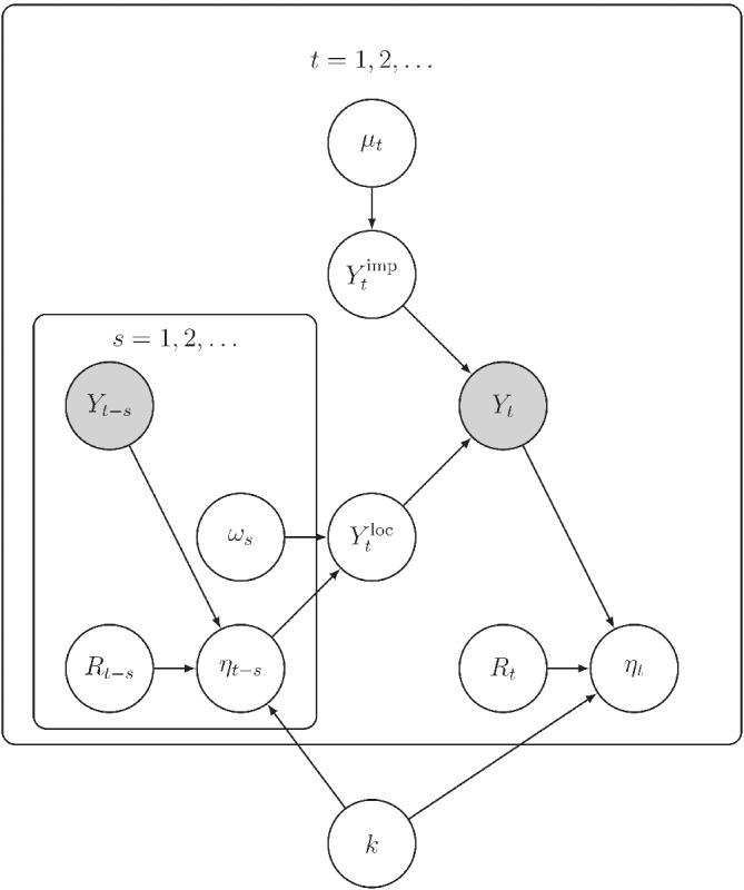
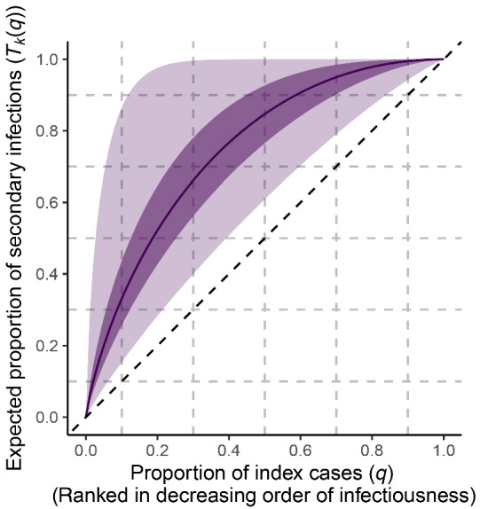
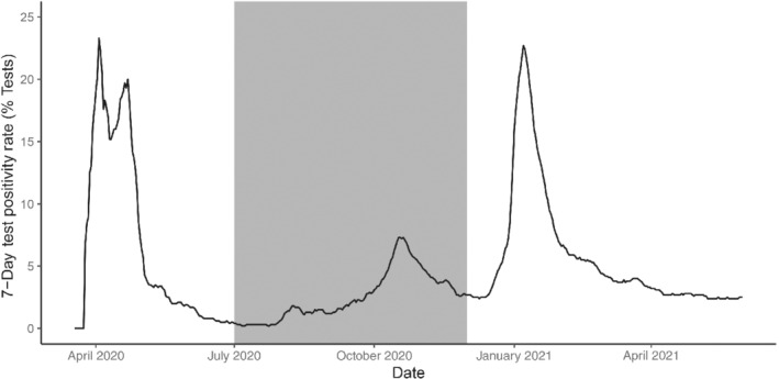
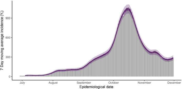
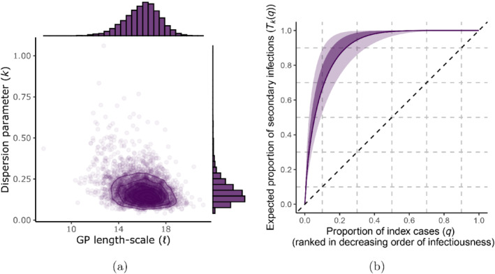
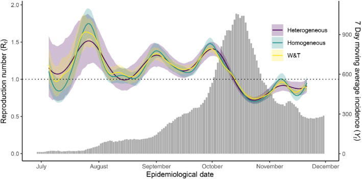
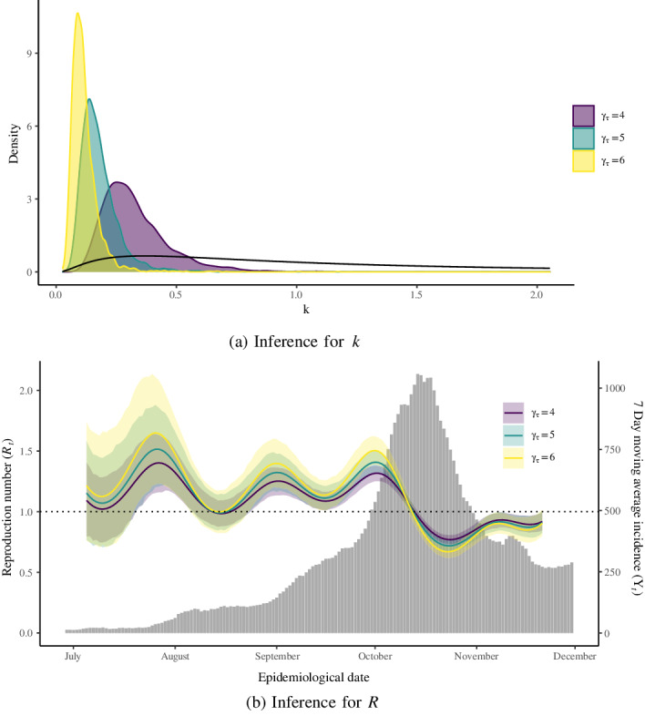
The expected number of secondary infections arising from each index case, referred to as the reproduction or $R$ number, is a vital summary statistic for understanding and managing epidemic diseases. There are many methods for estimating $R$ ; however, few explicitly model heterogeneous disease reproduction, which gives rise to superspreading within the population. We propose a parsimonious discrete-time branching process model for epidemic curves that incorporates heterogeneous individual reproduction numbers. Our Bayesian approach to inference illustrates that this heterogeneity results in less certainty on estimates of the time-varying cohort reproduction number $R_t$ . We apply these methods to a COVID-19 epidemic curve for the Republic of Ireland and find support for heterogeneous disease reproduction. Our analysis allows us to estimate the expected proportion of secondary infections attributable to the most infectious proportion of the population. For example, we estimate that the 20% most infectious index cases account for approximately 75%-98% of the expected secondary infections with 95% posterior probability. In addition, we highlight that heterogeneity is a vital consideration when estimating $R_t$ .

Keywords: branching processes; heterogeneous disease reproduction; time‐varying reproduction numbers.

FIGURE 1

A plate diagram of the conditional dependence structure within the generative model for epidemic curves described in Section 3.1, where only the epidemic curve $\dots ,Y_{-1},Y_0,Y_1\dots$ (shaded nodes) is observed. This figure highlights model parameters that are non‐identifiable from the epidemic curve alone. Even if the disease momentum ${\eta }_t$ was observed, joint inference for $R_t$ and $k$ depends on prior assumptions restricting the day‐to‐day variation in reproduction numbers.

FIGURE 2

The distribution of the expected proportion of secondary infections arising from the most infectious proportion of individuals in the population under a $\log k\sim 𝒩\left(0,1\right)$ prior for $k$, summarised by the the prior median (solid line), inter‐quartile range (dark shaded region), and 99% equal‐tailed interval (light shaded region). As an example, we see that this prior on $k$ provides support for 30%–95% of expected secondary infections arising from the most infectious 20% of index cases. [Colour figure can be viewed at wileyonlinelibrary.com]

FIGURE 3

The 7‐day test positivity rate as a percentage of all tests reported by the Health Protection Surveillance Centre up to June 2021. The shaded region covers the time period included in our analysis. Note that the test positivity never exceeds 10% in this period while it exceeds 20% at in April 2020 and January 2021. Our assumption is that a high positivity rate is indicative of a testing system that has been overwhelmed by cases, resulting in less reliable daily case counts.

FIGURE 4

The mean (solid line), 50% (dark shaded region), and 95% credible interval (light shaded region) for the posterior predictive distribution of the COVID‐19 epidemic curve in Ireland. Note that the predictive model is seeded by $N_0=5$ days. All observed daily case counts fall within the 95% credible interval of the posterior predictive distribution with 86% of counts within the 50% credible interval. [Colour figure can be viewed at wileyonlinelibrary.com]

FIGURE 5

(a) The sampled joint and marginal posterior distributions over $k$ and $\ell$. Each opaque point represents a sample, while contours are set to have a width of 0.3. We report 95% credible intervals for $k$ of $\left(0.07,0.33\right)$ and for $\ell$ of $\left(13,18\right)$. (b) The proportion of expected secondary infections attributable to the proportion $q$ of most infectious individuals. The mean (solid line), 50% (dark shaded region), and 95% credible interval (light shaded region) for this proportion over the interval $q\in \left[0,1\right]$ is presented. $T_k\left(q\right)$ is estimated numerically by Equation (13) given the posterior distribution for $k$. Based on this analysis we estimate, for example, that the 20% most infectious individuals give rise to 75%–98% of expected secondary infections with $95\%$ posterior probability, while 62%–82% of individuals are not expected to pass on the infection, again with $95\%$ posterior probability. [Colour figure can be viewed at wileyonlinelibrary.com]

FIGURE 6

The posterior mean (solid line) and 95% credible interval (shaded region) for $\mathit{R}$ under the heterogeneous, homogeneous and W&T model for disease transmission. At time points well supported by data, estimates for $R_t$ provided by each of the three methods show a general agreement. However, credible intervals under W&T or the assumption of homogeneous disease reproduction within each cohort are approximately 60% as wide as those in the heterogeneous case at each point in time. In addition, note that our estimate for $R_t$ is less ‘wiggly’ under heterogeneous disease transmission than in the homogeneous case. This behaviour illustrates that a more flexible model for $\mathit{R}$ is required to fit data when we assume homogeneous disease transmission. [Colour figure can be viewed at wileyonlinelibrary.com]

FIGURE B1

Summaries of the distribution for $\mathit{R}$ under a Gaussian process prior conditional on $R_0=R_N=1$ and ${\sigma }_f=1$ where $T=60$. Three prior specifications are considered: $\ell =10$ (a); $\ell =17.5$ (b); and $\ell =25$ (c). In each case the solid black line represents the conditional mean alongside the shaded 95% credible interval. Coloured lines represent samples from the conditional distribution. We note that smaller values for $\ell$ (shorter length‐scales) imply more flexible Gaussian process models. [Colour figure can be viewed at wileyonlinelibrary.com]

FIGURE C1

This analysis considers three candidate generation interval pmfs such that $\mathit{\omega }$ defined in (19) is parameterised by $({\gamma }_{\tau },{\sigma }_{\tau })\in \left\{(4,2),(5,2.5),(6,3)\right\}$. (a) presents the sampled posterior over $k$, while (b) presents posterior inference for $\mathit{R}$. We see that, while changes in $\omega$ do have an impact on inference, our overall conclusions on the heterogeneity of disease transmission remain broadly similar. [Colour figure can be viewed at wileyonlinelibrary.com]

References

-
- Anderson, R.M. & May, R.M. (1992) Infectious diseases of humans: dynamics and control. Oxford: Oxford University Press.
- Becker, N.G. & Britton, T. (1999) Statistical studies of infectious disease incidence. Journal of the Royal Statistical Society: Series B (Statistical Methodology), 61(2), 287–307.
LinkOut - more resources
Full Text Sources