A single-cell transcriptional timelapse of mouse embryonic development, from gastrula to pup

Abstract

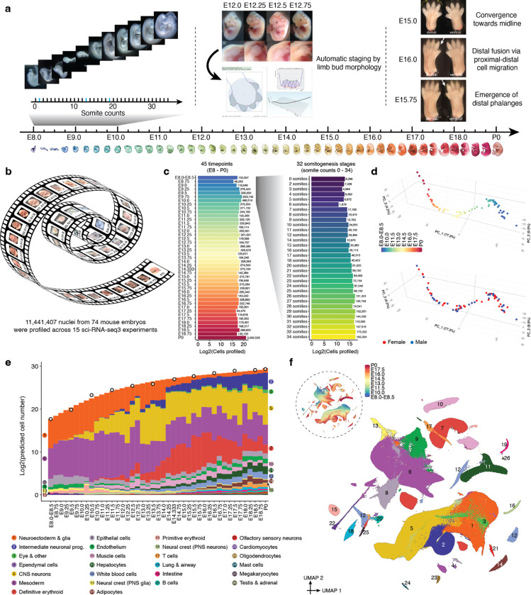
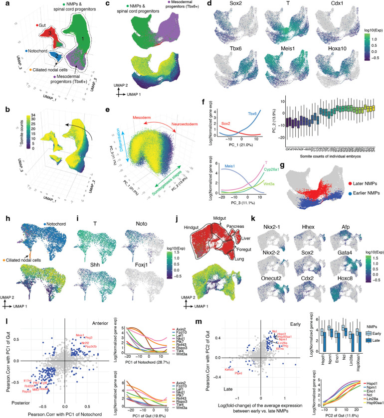
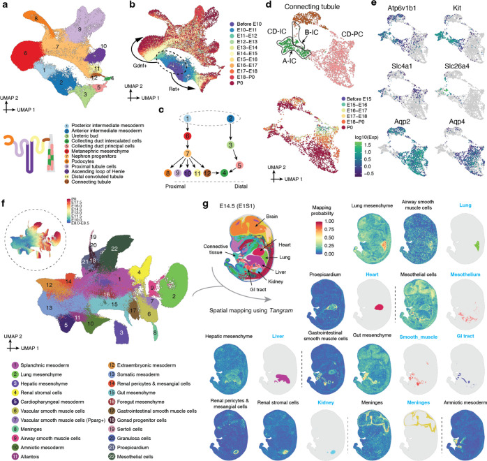
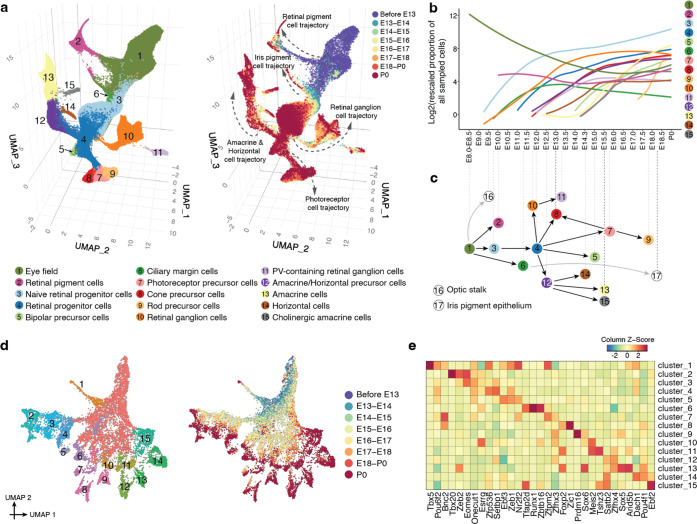
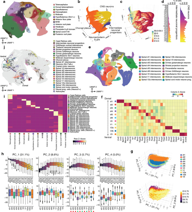
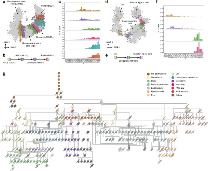
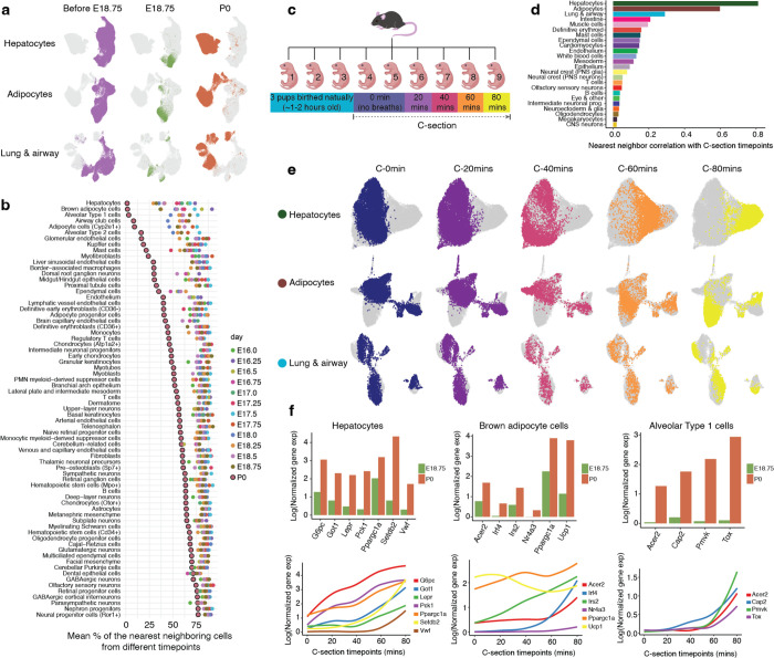
The house mouse, Mus musculus, is an exceptional model system, combining genetic tractability with close homology to human biology. Gestation in mouse development lasts just under three weeks, a period during which its genome orchestrates the astonishing transformation of a single cell zygote into a free-living pup composed of >500 million cells. Towards a global framework for exploring mammalian development, we applied single cell combinatorial indexing (sci-*) to profile the transcriptional states of 12.4 million nuclei from 83 precisely staged embryos spanning late gastrulation (embryonic day 8 or E8) to birth (postnatal day 0 or P0), with 2-hr temporal resolution during somitogenesis, 6-hr resolution through to birth, and 20-min resolution during the immediate postpartum period. From these data (E8 to P0), we annotate dozens of trajectories and hundreds of cell types and perform deeper analyses of the unfolding of the posterior embryo during somitogenesis as well as the ontogenesis of the kidney, mesenchyme, retina, and early neurons. Finally, we leverage the depth and temporal resolution of these whole embryo snapshots, together with other published data, to construct and curate a rooted tree of cell type relationships that spans mouse development from zygote to pup. Throughout this tree, we systematically nominate sets of transcription factors (TFs) and other genes as candidate drivers of the in vivo differentiation of hundreds of mammalian cell types. Remarkably, the most dramatic shifts in transcriptional state are observed in a restricted set of cell types in the hours immediately following birth, and presumably underlie the massive changes in physiology that must accompany the successful transition of a placental mammal to extrauterine life.

Figure 1.. A single cell transcriptional timelapse of mouse development, from gastrula to pup.

a, Embryos were collected and precisely staged based on morphological features, including by counting somite numbers (up to E10) and an automated process that leverages limb bud geometry (E10-E15) (Methods). Each embryo was assigned to one of 45 temporal bins at 6-hr increments from E8 to P0, and to more highly resolved 2-hr bins at earlier timepoints based on somite counts. The first three bins (E8.0, E8.25, E8.5) are combined for presentation purposes, and this is also the subset of the data that was previously reported. Embryos with somite counts 1, 3, 19 are missing from the series (blue ticks in sub-axis at left). See Supplementary Figs. 1–2 and Supplementary Table 1 for further details. b, Across 15 sci-RNA-seq3 experiments, we generated single nucleus profiles for 11.4M cells from 74 embryos spanning mouse development from late gastrulation to birth, with around 2-hr temporal resolution from 0 to 34 somites, and 6-hr resolution through to birth. c, The number (log2 scale) of nuclei profiled at each timepoint, shown for 6-hr bins at left and for 2-hr bins (somitogenesis) at right. d, Embeddings of pseudo-bulk RNA-seq profiles of 74 mouse embryos in PCA space with visualization of top three PCs. Briefly, single nucleus data from each embryo was aggregated to create 74 profiles, with which we performed dimensionality reduction via PCA. Embryos are colored by either developmental stage (top) or data-inferred sex (bottom). e, Composition of embryos from each 6-hr bin by major cell cluster. The y-axis is scaled to the estimated cell number (log2 scale) at each timepoint (Methods). Briefly, we isolated and quantified total genomic DNA from whole embryos to estimate the total cell number at each of 12 stages, spanning from E8.5 to P0 (1-day bins, highlighted by black circles), and then applied polynomial regression to predict log2-scaled cell number of the whole embryo at each of the 43 timepoints (P0 was treated as E19.5 in the regression). CNS: central nervous system. PNS: peripheral nervous system. f, 2D UMAP visualization of the whole dataset. Colors and numbers correspond to 26 major cell cluster annotations as listed in the key of panel e. Dashed circle inset at top left shows the same UMAP colored by developmental stage (plotting a uniform number of cells per timepoint).

Figure 2.. Transcriptional heterogeneity in the posterior embryo during the early somitogenesis.

a, Re-embedded 3D UMAP of 121,118 cells which were initially annotated as neuromesodermal progenitors (NMPs) & spinal cord progenitors, mesodermal progenitors (Tbx6+), notochord, ciliated nodal cells, or gut, from embryos during the early somitogenesis (somite counts 0–34; E8-E10). Cells are colored by their initial annotations. Three clusters are identified and highlighted, with cluster 1 dominated by NMPs and their derivatives, cluster 2 dominated by notochord and ciliated nodal cells, and cluster 3 dominated by gut. b, The same UMAP as in panel a, colored by somite counts. Arrow highlights the increment of somite counts. c, Re-embedded 2D UMAP of cells from cluster 1 in panel a. Cells are colored by either their initial annotations (top) or somite counts (bottom). d, The same UMAP as in panel c, colored by gene expression of marker genes which appear specific to different subpopulations of NMPs: column 1: differences between neuroectodermal (Sox2+) vs. mesodermal (Tbx6+) fates; column 2: the differentiation of bipotential NMPs (T+, Meis1−) towards either fate^,; column 3: earlier (Cdx1+) vs. later (Hoxa10+) NMPs. e, 3D visualization of the top three principal components (PCs) of gene expression variation in cells from cluster 1, calculated on the basis of the 2,500 most highly variable genes. Cells are colored by the somite count of the embryo from which they derived. As further shown in panel f, PC1 correlates with mesodermal vs. neuroectodermal fates (red arrow), PC2 with somite stage (green arrow), and PC3 with the progression of differentiation of bipotential NMPs towards either fate (blue arrow). f, Correlations between top three PCs and the normalized expression of selected genes (Sox2 & Tbx6 for PC1; T, Cyp26a1, Wnt3a and Meis1 for PC3) or somite counts (for PC2). Gene expression values were calculated from original UMI counts normalized to total UMIs per cell, followed by natural-log transformation. The line of gene expression was plotted by the geom_smooth function in ggplot2. In the boxplot, the center lines show the medians; the box limits indicate the 25th and 75th percentiles. The genes significantly correlated with each PC are shown in Supplementary Table 6. g, The same UMAP as in panel c, with earlier (blue, n = 4,949 cells) and later (red, n = 3,910 cells) NMPs highlighted. Here cells are labeled as NMPs if they are both strongly T+ (raw count >= 5) & Meis1− (raw count = 0). h, Re-embedded 2D UMAP of cells from cluster 2 in panel a. Cells are colored by either the initial annotation (top) or somite counts (bottom). i, The same UMAP as in panel h, colored by gene expression of marker genes which appear specific to notochord (T+, Noto+, Shh+)^, or ciliated nodal cells (Foxj1+). j, Re-embedded 2D UMAP of cells from cluster 3 in panel a. Cells are colored by either the initial annotations (top) or somite counts (bottom). Different subpopulations of gut cells are highlighted by black circles. k, The same UMAP as in panel j, colored by gene expression of marker genes which appear specific to different subpopulations of gut cells, including lung (Nkx2–1+), hepatocytes (Hhex+, Afp+)^,, pancreas (Nkx2–2+), foregut (Gata4+, Sox2+)^,, midgut (Gata4+, Onecut2+)^,, and hindgut (Cdx2+, Hoxc8+)^–. l, On the left, the Pearson correlation coefficient between gene expression for the top highly variable genes and either PC1 of notochord (x-axis) or PC1 of gut (y-axis). For each cell cluster, the top 2,500 highly variable genes were identified and their gene expression values were calculated from original UMI counts normalized to total UMIs per cell, followed by natural-log transformation and scaling. After performing Pearson correlation with the selected PC, significant genes were identified if their correlation coefficients are < mean − 1 standard deviation or > mean + 1 standard deviation of all the correlation coefficients, and FDR < 0.05. The overlapped genes between two cell clusters are shown as each dot, and the overlapped significant genes highlighted in blue. The first quadrant corresponds to the inferred anterior aspect of each cluster, while the third quadrant corresponds to the inferred posterior aspect. On the right, gene expression of selected genes involved in Wnt signaling are plotted over PC1 of notochord (top) or PC1 of gut (bottom). Gene expression values were calculated from original UMI counts normalized to total UMIs per cell, followed by natural-log transformation. The line of gene expression was plotted by the geom_smooth function in ggplot2. m, On the left, the log-scaled fold-change of the average expression for the top highly variable genes between early vs. late NMPs (x-axis), and the Pearson correlation coefficient between gene expression for the top highly variable genes and PC2 of gut (y-axis). The first quadrant is associated with early somite counts for each cluster, while the third quadrant is associated with late somite counts. On the right, gene expression of selected genes (several Myc targets, Lin28a, Hsp90aa1) are plotted between early vs. late NMPs (top) or over PC2 of gut (bottom). The highly differentially expressed genes between early vs. late NMPs were identified using the FindMarkers function of Seurat/v3, after filtering out genes that are detected in < 10% of cells in both of the two populations. Significant genes were identified if their absolutely log-scaled fold-changes > 0.25, and adjusted p-values < 0.05.

Figure 3.. Diversification of the intermediate and lateral plate mesoderm.

a, Re-embedded 2D UMAP of 95,226 cells corresponding to renal development. A schematic of a nephron is shown at the bottom left. b, The same UMAP as in panel a, colored by developmental stage (after downsampling to a uniform number of cells per time window). Dashed circle highlights posterior & anterior intermediate mesoderm, with arrows highlighting derivative trajectories expressing Gdnf and Ret, respectively. c, Manually inferred relationships between annotated renal cell types. Label annotations in panel a. Dashed circle highlights posterior & anterior intermediate mesoderm. Dashed line highlights the expected spatial ordering of annotated cell types from proximal (left) to distal (right) aspect of nephron. d, Re-embedded 2D UMAP of 2,894 cells from connecting tubule cells, collecting duct principal cells (CD-PC), and collecting duct intercalated cells (CD-IC). Cells are colored by either their initial annotations (top) or timepoint (bottom). Black circles highlight the cells which appear to be either type A (A-IC) or type B (B-IC) intercalated cells. e, The same UMAP as in panel d, colored by expression of marker genes specific to CD-IC (Atp6v1b1+), A-IC (Kit+, Slc4a1+), B-IC (Slc26a4+), CD-PC (Aqp2+, Aqp4+), and connecting tubule (Aqp2+, Aqp4-) ^,. f, Re-embedded 2D UMAP of 745,494 cells from lateral plate & intermediate mesoderm derivatives. Dashed circle at the top left highlights the same UMAP with cells colored by developmental stage. g, To infer the spatial origin of each lateral plate & intermediate mesoderm derivative shown in panel f, we leveraged a public dataset, Mosta, which profiles spatial transcriptomes for 53 sections of mouse embryos spanning 8 timepoints from E9.5 to E16.5, together with our data and the Tangram algorithm. In brief, for each timepoint of the Mosta data, we combined scRNA-seq data from three adjacent timepoints from our data (e.g. E16.25, E16.5, and E16.75 from scRNA-seq vs. E16.5 from Mosta data), and the total number of voxels within each section was randomly downsampled to 9,000 for computational efficiency. After applying Tangram, for each section, a cell-by-voxel matrix with mapping probabilities was returned. To reduce noise, we further smoothed the mapping probabilities for each voxel by averaging values of their k nearest neighboring voxels (k is calculated by natural-log scaled total number of voxels on that section) followed by scaling it to 0→1 across voxels of each section. An image of one selected section (E1S1) from E14.5 of the Mosta data is shown on the top left with major regions labeled. The spatial mapping probabilities across voxels on this section for selected subtypes within the lateral plate & intermediate mesoderm derivatives are shown (black titles), with the regional annotation appearing to best correspond to the inferred spatial pattern shown alongside (blue titles). The mapping results for the other sections are provided here.

Figure 4.. The timing and trajectories of retinal development.

a, Re-embedded 3D UMAP of 160,834 cells corresponding to the retinal development from E8 to P0. Cells are colored by either their initial annotations (left) or timepoint (right, after downsampling to a uniform number of cells per time window). Arrows highlight five of the main trajectories observed. b, Rescaled proportion of profiled cells (log2; y-axis) for each cell type shown in panel a, as a function of developmental time (x-axis). For rescaling, the % of profiled cells in the entire embryo assigned a given annotation was multiplied by 100,000, prior to taking the log2. Line plotted with geom_smooth function in ggplot2. c, Schematic of retinal cell types emphasizing the timing at which they first appear and their inferred developmental relationships from E8-P0. The gray lines indicate subsets of the eye field and RPE subsequently annotated as the optic stalk (label 16) and iris pigment epithelium (label 17), respectively. Cell types are positioned along the x-axis at the timepoint at which they are first observed (Supplementary Fig. 10e). d, Re-embedded 2D UMAP of retinal ganglion cells. Cells are colored by either clusters (left; Leiden clustering followed by downselection to late-appearing clusters) or timepoint (right). e, The top 3 TF markers of the 15 clusters shown in panel d. Marker TFs were identified using the FindAllMarkers function of Seurat/v3. Their mean gene expression values in each cluster are represented in the heatmap, calculated from original UMI counts normalized to total UMIs per cell, followed by natural-log transformation. The full list of significant TFs is provided in Supplementary Table 14.

Figure 5.. The emergence of neuronal subtypes from the patterned neuroectoderm.

Please note panels are arranged in a clockwise manner. a, Re-embedded 2D UMAP of 1,185,052 cells, corresponding to different neuroectodermal territories, from neuroectoderm & glia major cell clusters from stages <E13. Derived cell types, e.g. eye field, glia, neurons, are excluded. b, Re-embedded 3D UMAP of 1,772,567 cells from neuroectodermal territories together with derived cell types, from stages <E13. Derived cell types are mainly from the CNS neuron, ependymal cell (more specifically, choroid plexus), and intermediate neuronal progenitor cell clusters. c, The same UMAP as in panel b, colored by timepoint. d, Composition of embryos from each 6-hr bin by intermediate neuronal progenitor (left) and CNS neuron (right) major cell clusters. e, Re-embedded 2D UMAP of 296,020 cells (glutamatergic neurons, GABAergic neurons, spinal cord dorsal progenitors, and spinal cord ventral progenitors) from stages <E13. f, The top 3 TF markers of the 11 spinal interneurons. Each spinal interneuron was first randomly downsampled to 10,000 cells and marker TFs were identified using the FindAllMarkers function of Seurat/v3. Their mean gene expression values in each cluster are represented in the heatmap, calculated from original UMI counts normalized to total UMIs per cell, followed by natural-log transformation. The full list of significant TFs is provided in Supplementary Table 15. g, 3D visualization of the top three PCs of gene expression variation in 11 spinal interneurons (after randomly downsampling each spinal interneuron to 10,000 cells), calculated on the basis of the 2,500 most highly variable genes. Cells are colored by either cell types (top) or timepoints (bottom). h, Correlations between top four PCs and timepoints (top row) or cell types (bottom row). In the boxplots, the center lines show the medians; the box limits indicate the 25th and 75th percentiles. The red triangles and green stars highlight spinal cord interneurons which are glutamatergic vs. GABAergic identity, respectively. i, The number of mutual nearest neighbors (MNN) pairs between pairwise neuroectodermal territories (column) and their derivative cell types (row). The cell populations as shown in panel b, are first embedded into 30 dimensional PCA space, and then for individual derivative cell types, the MNN pairs (k = 10 used for k-NN) between their earliest 500 cells and the cells from neuroectodermal territories are identified. A handful of derivative cell types with <500 cells are excluded. Three derivative cell types with fewer than 50 MNN pairs are excluded but further analyzed by iterative mapping (Supplementary Fig. 14a). j, The same UMAP as in panel a, but with inferred progenitor cells colored by derivative cell type with the most frequent MNN pairs. Dotted circles highlight the dorsal and ventral spinal interneuron neurogenesis domains of the hindbrain & spinal cord.

Figure 6.. A data-driven tree relating cell types throughout mouse development, from zygote to pup.

a, Illustration of basis for edge inference heuristic. Re-embedded 2D UMAP of 101,001 cells from hematopoietic stem cells (Cd34+), hematopoietic stem cells (Mpo+), monocytic myeloid-derived suppressor cells (MDSCs), and PMN myeloid-derived suppressor cells (MDSCs) within the “Blood” subsystem. Cells involved in MNN pairs that bridge cell types are coloured. For example, hematopoietic stem cells (Cd34+) and hematopoietic stem cells (Mpo+) involved in MNN pairs between these two cell types are coloured yellow and light purple, respectively. b, Inferred lineage relationships between annotated cell types in panel a, with corresponding color scheme. c, The % of inter-cell-type MNN cells (y-axis) over the total number of cells profiled from embryos from the corresponding time bin, with the same color scheme as panels a & b. d, Additional illustration of basis for edge inference heuristic. Re-embedded 2D UMAP of 71,718 cells from gut, lung progenitor cells, and alveolar Type 2 cells within the “Gut” subsystem. Cells involved in MNN pairs that bridge cell types are coloured. For example, gut and lung progenitor cells involved in MNN pairs between these two cell types are coloured yellow and light purple, respectively. e, Inferred lineage relationships between annotated cell types in panel d, with corresponding color scheme. f, The % of inter-cell-type MNN cells (y-axis) over the total number of cells profiled from embryos from the corresponding time bin, with the same color scheme as panels d & e. g, A rooted, directed graph corresponding to a mouse development, spanning E0 to P0 (yFiles Hiearchic layout in Cytoscape/v3.9.1). For presentation purposes, most ‘spatial continuity’ edges are removed (except for those between spinal cord dorsal & ventral progenitors (after E13.0) and GABAergic & glutamatergic neurons (after E13.0)). We also merged nodes with redundant labels derived from different datasets (i.e. “dataset equivalence” edges), resulting in a rooted graph composed of 262 cell type nodes and 338 edges. Nodes are colored and labeled by each of the 14 subsystems: Pre-gastrulation (n = 2,250 cells), Gastrulation (n = 108,857 cells), Blood (n = 1,576,789 cells), Brain & spinal cord (n = 4,434,234 cells), Endothelium (n = 312,029 cells), Epithelial cells (n = 398,373 cells), Eye (n = 166,852 cells), Gut (n = 453158 cells), Lateral plate mesoderm (n = 992,903 cells), Mesoderm (n = 2,717,903 cells), Notochord (n = 3,812 cells), PNS glia (n = 126,743 cells), PNS neurons (n = 146,825 cells), and Kidney (n = 111,786 cells).

Figure 7.. Rapid shifts in transcriptional state occur in a restricted subset of cell types upon birth.

a, Re-embedded 2D UMAP of cells from three major cell clusters: hepatocytes (top row), adipocytes (middle row), and lung & airway (bottom row). For each row, the same UMAP is shown three times, with colors highlighting cells from before E18.75 (left), E18.75 (middle), or P0 (right) embryos. b, To systematically identify which cell types exhibit abrupt transcriptional changes before vs. after birth, for each of the 190 cell types, cells from animals harvested subsequent to E16 were combined, followed by PCA based on the top 2,500 highly variable genes. The 71 cell types with >= 200 cells from P0 and >= 200 cells from at least five timepoints prior to P0 were retained for the following analysis. First, timepoints with >= 200 cells were selected followed by downsampling cells from each timepoint to the median number of cells across those selected timepoints. Then, individual cells were searched for k-nearest neighbors (k was adjusted for different cell types, by taking log2-scaled median number of cells across the selected timepoints) in PCA space (n = 30 dimensions). Finally, for cells within each cell type, the average proportions of their nearest neighbor cells that are from a different timepoint were calculated. In this framing, a low proportion of neighbors from different timepoints corresponds to a relatively abrupt change in transcriptional state. Points corresponding to P0 are highlighted with black boundary. c, A new scRNA-seq dataset (hereafter referred to as “birth-series”) was generated from nuclei derived from nine individual pups from a single litter harvested shortly after delivery. This includes three vaginally birthed pups and six C-section delivered pups with 20 min increments between delivery and harvesting. d, For each major cell cluster in the birth-series dataset, we took cells from the six pups delivered by C-section and calculated a Pearson correlation coefficient between the timepoint of each cell and the average timepoints of its 10 nearest neighbors identified from the global PCA embedding (n = 30 dimensions). In this framing, high correlations are consistent with rapid, synchronized changes in transcriptional state. e, Re-embedded 2D UMAP of cells from three major cell clusters, based on cells from six pups delivered by C-section in birth series dataset: hepatocytes (n = 41,122 cells, top row), adipocytes (n = 19,696 cells, middle row), and lung & airway (n = 7,986 cells, bottom row). For each row, the same UMAP is shown multiple times, with colors highlighting cells from pups harvested after different intervals after delivery. f, Average normalized gene expression of selected genes are plotted between E18.75 vs. P0 in the original data (top), and normalized gene expression of the same genes are plotted as a function of C-section timepoints (bottom), for hepatocytes (left column), brown adipocyte cells (middle column), and alveolar type 1 cells (right column), respectively. Gene expression values were calculated from original UMI counts normalized to total UMIs per cell, followed by natural-log transformation. The line of gene expression was plotted by the geom_smooth function in ggplot2.

References

1. Packer J. S. et al. A lineage-resolved molecular atlas of C. elegans embryogenesis at single-cell resolution. Science 365, (2019). - PMC - PubMed
1. Calderon D. et al. The continuum of Drosophila embryonic development at single-cell resolution. Science 377, eabn5800 (2022). - PMC - PubMed
1. Farrell J. A. et al. Single-cell reconstruction of developmental trajectories during zebrafish embryogenesis. Science 360, (2018). - PMC - PubMed
1. Wagner D. E. et al. Single-cell mapping of gene expression landscapes and lineage in the zebrafish embryo. Science 360, 981–987 (2018). - PMC - PubMed
1. Briggs J. A. et al. The dynamics of gene expression in vertebrate embryogenesis at single-cell resolution. Science 360, (2018). - PMC - PubMed
Publication types