The proteomic landscape of genome-wide genetic perturbations

Abstract

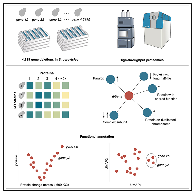
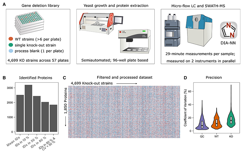
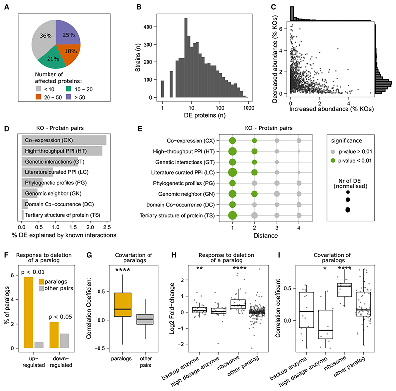
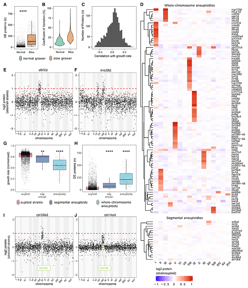
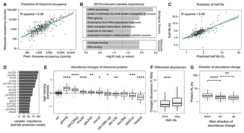
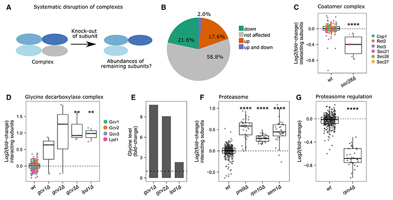
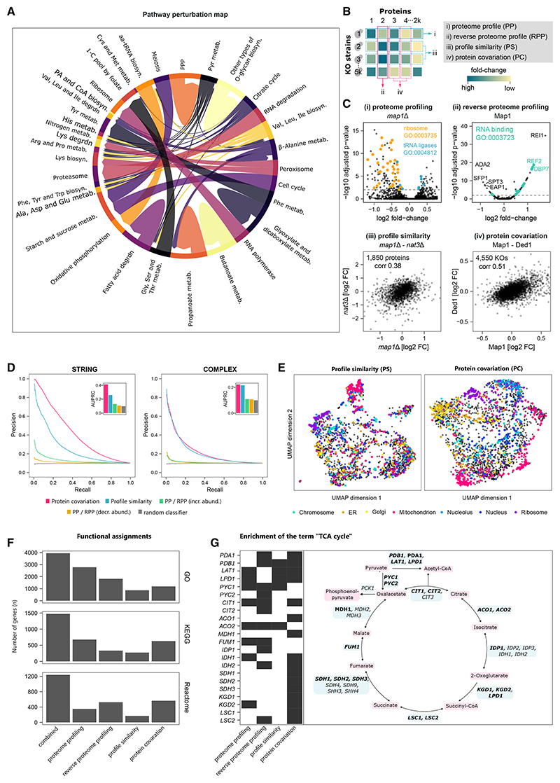
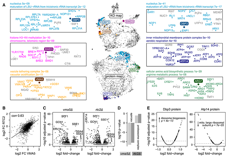
Functional genomic strategies have become fundamental for annotating gene function and regulatory networks. Here, we combined functional genomics with proteomics by quantifying protein abundances in a genome-scale knockout library in Saccharomyces cerevisiae, using data-independent acquisition mass spectrometry. We find that global protein expression is driven by a complex interplay of (1) general biological properties, including translation rate, protein turnover, the formation of protein complexes, growth rate, and genome architecture, followed by (2) functional properties, such as the connectivity of a protein in genetic, metabolic, and physical interaction networks. Moreover, we show that functional proteomics complements current gene annotation strategies through the assessment of proteome profile similarity, protein covariation, and reverse proteome profiling. Thus, our study reveals principles that govern protein expression and provides a genome-spanning resource for functional annotation.

Keywords: Saccharomyces cerevisiae; data-independent acquisition; deletion; functional genomics; functional proteomics; gene annotation; high throughput; knockout; quantitative proteomics; systems biology.

Graphical abstract

Figure 1. Quantitative proteomes for the genome-scale yeast gene-deletion collection

(A) Experimental setup (STAR Methods). (B) Protein identification numbers as mean per sample (2,520), identified in 10% of the samples (3,205), identified in 50% of the samples (2,445), identified in 80% of the samples (2,036), and identified in 80% of the WT samples with CV <50% (filtered dataset as described in STAR Methods) (1,850). All values were calculated for samples that passed the quality control (QC) thresholds. (C) The filtered quantitative data are shown as a heatmap with 1,850 unique proteins measured across the 4,699 KOs, containing 8,693,150 protein quantities. (D) The coefficients of variation (CVs; in %) were calculated for each protein and are shown for pooled yeast digest samples (QC, n = 389), whole-process control samples (WT, n = 388), and KO samples (KO, n = 4,699). Median CV values are 8.1% across the technical replicates of a pooled digest, 11.3% across the biological replicates of the wild-type strain, and 16.2% across the KO library. CVs were calculated on the filtered dataset and are shown from 0% to 70% (see Figure S1B for all data points).

Figure 2. The proteomic response to systematic gene deletion

(A) Fraction of gene deletion strains (n = 4,699) in which proteins are differentially expressed (STAR Methods). (B) Distribution of proteomic responses, given as the number of differentially expressed proteins (DE; Benjamini-Hochberg (BH)-adjusted p value < 0.01). (C) Increased and decreased abundance of each protein across the 4,699 KO strains are given as dots and as histograms. (D) Differentially expressed proteins upon gene deletions were compared with physical, genetic, or functional interactions, collected as part of the YeastNet resource (v3). (E) Differential abundance of proteins is related to their distance to the deleted gene in the indicated network. Differentially abundant proteins of distance i were normalized to the total number of proteins of distance i within the respective network. A significant enrichment (hypergeometric test, p value < 0.01) is indicated by color. (F) Percentage of paralogs from whole-genome duplications (ohnologs) that have increased or decreased abundance (BH-adjusted p value < 0.01) after the deletion of one of the paralog partners (yellow). The number of increased or decreased proteins across all KOs is shown as a gray bar for reference. (G) Spearman correlation coefficients are shown for ohnologs (n = 107 pairs) and for all other protein pairs (n = 1,710,215). The median correlation coefficients are 0.19 and 0.01 for paralogs and other pairs, respectively (Wilcoxon signed-rank test; ****p value ≤ 0.0001). (H) paralogs were classified as compensatory enzymes (backup); enzymes duplicated to increase gene dosage; or protein components of the ribosome (according to the GO term “structural constituent of ribosome”), and compared with measured paralogs not categorized according to these groups (“other paralogs”) (**p value ≤ 0.01; ****p value ≤ 0.0001, Student’s t test). (I) Correlation coefficients are based on Spearman rank coefficients and compared to measured paralogs not categorized (“other paralogs”) (*p value ≤ 0.05; ****p value ≤ 0.0001; Student’s t test). See also Figure S2.

Figure 3. The effect of growth and chromosomal copy-number variations (aneuploidies) on the proteome

(A) Numbers of differentially expressed proteins in slow-growing KO strains (n = 748) and normal growers (n = 3,930). ****p value ≤ 0.0001 (Wilcoxon signed-rank test). (B) The proteome dispersion within slow-growing strains is compared with the dispersion within normal-growing strains and is given as protein coefficients of variations (in %). The CV values are shown for CV < 100%. (C) Correlation coefficients (Pearson correlation) are shown as histograms for all pairwise protein-abundance-growth correlations. (D) Median log₂ protein abundance levels (normalized, see STAR Methods) are shown for each chromosome. (E and F) Protein abundances, sorted by their chromosomal location, are shown for dbf2Δ and kre28Δ, respectively (Manhattan plot). (G) The normalized growth rates are compared between euploid (n = 4,428, median = 0.97), segmental aneuploidy (n = 18, median = 0.90), and whole-chromosomal aneuploidy strains (n = 84, median = 0.65) (Wilcoxon signed-rank test; **p value ≤ 0.01; ****p value ≤ 0.0001). (F) The numbers of significantly changed proteins are compared between euploid (n = 4,428, median = 16), segmental aneuploidy (n = 18, median = 74), and whole-chromosomal aneuploidy strains (n = 84, median = 208) (Wilcoxon signed-rank test; ****p value ≤ 0.0001). (I and J) Protein abundances, sorted by their chromosomal location, are shown for rpl16bΔ and rpl14aΔ, respectively. See also Figure S3.

Figure 4. The interdependency of differential protein expression with translation rate and turnover

(A) Ribosomal occupancies are predicted with an elastic net model. The model was trained on 80% of the proteins (n = 1,392) and applied on the remaining 20% of the proteins (test set, n = 346). The plot shows only proteins from the test set. Ribosomal occupancies were taken from a reference dataset and log₁₀-transformed. The proteome data were log₂ transformed, centered, and scaled. (B) Gene Ontology (GO) slim term enrichment analysis of the top features selected by the model using a Fisher’s exact test (STAR Methods). (C) Half-lives are predicted with an elastic net model. The model was trained on 80% of the proteins (n = 1,398) and applied on the remaining 20% of the proteins (test set, n = 348). The plot only shows proteins from the test set. Half-lives were taken from a reference dataset and log₁₀ transformed. The proteome data were log₂ transformed, centered, and scaled. (D) The 15 most important KO strains in the regression model for half-lives. The KO strains are ranked by importance and scaled to have a maximum value of 100. (E) Abundance of ribosomal 60S subunit proteins in 10 KO strains that were selected as the most important feature for the prediction of protein half-life. Protein intensities are centered and log₂-transformed. Significance for the comparison to the WT abundance levels (two-sided t test) is shown with asterisks (****p ≤ 0.0001; ***p ≤ 0.001; **p ≤ 0.01; *p ≤ 0.05; ^nsp > 0.05). (F) Differential abundance of proteins with short (below median) and long (above median) half-lives (****p ≤ 0.0001, Wilcoxon signed-rank test). (G) Half-lives (in h, log₁₀ transformed) are shown as boxplots for proteins that are predominantly decreased in abundance, increased in abundance, or change in both directions across the KO strains. Directionality was defined as ratios of increased and decreased abundance changes being >75% and <25% quantile for down and up, respectively. Significance (two-sided Wilcoxon signed-rank test with “no direction” as a reference) is shown with asterisks (****p value ≤ 0.0001; **p value ≤ 0.01). See also Figure S4.

Figure 5. The response of protein complexes to genome-wide perturbation

(A) Scheme: the response of complex subunits to the deletion of one subunit. (B) Fraction of complexes in which at least one deletion of a subunit induces a decrease (22%, green), increase (18%, orange), or in which some deletions induce increase and others decrease (2%, purple) of subunit abundances. The total number of considered complexes is 51 (STAR Methods). (C) Relative abundances of the coatomer complex subunits Cop1, Ret2, Ret3, Sec21, Sec26, and Sec27 are compared between sec28Δ and WT samples. Data are centered and log₂-transformed. (D) Relative abundances of the glycine decarboxylase complex subunits Gcv1, Gcv2, Gcv3, and Lpd1 are shown for the KOs of the glycine decarboxylase complex (gcv1Δ, gcv2Δ, gcv3Δ, and lpd1Δ) and WT samples. (E) Relative glycine abundances in glycine decarboxylase KOs (gcv1Δ, gcv2Δ, and lpd1Δ) are shown, as derived from a reference dataset. (F) The relative protein abundances of proteasome complex subunits in the viable KOs of the proteasome complex—pre9Δ, rpn10Δ, and sem1Δ—compared with their abundance levels in WT strains. Data are centered and log₂-transformed. (G) The relative protein abundances of all measured proteasome subunits in rpn4Δ are compared with their WT abundance levels. Significance (two-sided Student’s t test with WT as a reference) is shown with asterisks (**** for p value ≤ 0.0001; *** for p value ≤ 0.001; ≤ for p value ≤ 0.01; * for p value ≤ 0.05).

Figure 6. Annotating gene functions using functional proteomics

(A) Map connecting genetic perturbations to the corresponding proteome response. Genes are grouped by KEGG pathway,^, arrows point from perturbed toward affected pathways (STAR Methods). PPP, pentose phosphate pathway; metab., metabolism; biosyn., biosynthesis; degrdn, degradation; 1-C, one carbon; PA, pantothenate; aa, aminoacyl; Pyr, pyruvate; amino acids indicated by standard three-letter code. (B) The four functional annotation strategies supported by this dataset. (C) The MAP1 gene exemplifies the complementary nature of these proteome annotation strategies. (Ci and Cii) Volcano plots of proteome profile and reverse proteome profile of the map1Δ strain and Map1 protein, respectively. Dashed lines indicate significant changes (adjusted p value < 0.01). (Ciii) Protein fold-changes (FC) measured in the map1Δ strain are similar to those in the nat3Δ strain (Spearman correlation = 0.38). (Civ) Abundance changes of Map1 and Ded1 proteins are correlated across all strains (Spearman correlation = 0.51). (D) Precision-recall analyses showing that profile similarities (PSs) and protein covariation (PC) capture gene function very well. In addition, protein-KO pairs were ranked by the protein fold-change in the KO, showing that the extent of upregulation (PP/RPP [incr. abundance]) or downregulation (PP/RPP [decr. abundance]) is a relatively poor indicator of shared protein/KO function. Performance was assessed using two gold standards for shared protein function, STRING (left) and COMPLEAT protein complexes (right). Only responsive KOs were considered for profile similarity analysis. See STAR Methods for details. (E) Functional maps created using uniform manifold approximation and projection (UMAP), grouping KO strains by profile similarity (left) and proteins by covariation (right). Subcellular compartment annotation shows that both approaches capture subcellular organization. (F) Number of genes that could be associated with at least one GO term, KEGG pathway or Reactome pathway by over-representation analysis. For PPs, the enrichment was performed on the differentially expressed proteins in each strain and for RPPs the KOs in which the respective protein was differentially expressed. For PS and PC, we considered the highest-scoring 1% of associations in the networks. Functional enrichment was considered significant for p < 0.01 (topology-weighted topGO analysis) or BH-adjusted p < 0.01 (KEGG/Reactome Fisher’s exact test, STAR Methods). (G) Functional annotations capture known interactions within the TCA cycle. The KEGG term “TCA cycle” was enriched in 22 TCA cycle genes by at least one of the annotation methods, 6 by two methods, and 6 by three. See also Figure S5.

Figure 7. Exploring functional relationships in a proteomic map of genome-scale perturbation

(A) Proximity in the UMAPs of KO strains and proteins reflects functional similarity. Three KOs (top map/left panel) and three proteins (bottom map/right panel) are shown as examples. KOs/proteins that are strongly linked to the example gene (within 1% highest-scoring associations, STAR Methods) are highlighted in color. Selected GO terms enriched among these groups are indicated (enrichment p value from Fisher’s exact test). (B) Protein fold-changes (FC) of two KOs that are near each other in the UMAP (vma5Δ and rtc2Δ, bottom left in A) are strongly correlated (biweight midcorrelation coefficient = 0.63). (C) Volcano plots of the PPs of the same KOs, revealing many overlapping differentially expressed proteins, a few of which are labeled. (D) GO term enrichment for differentially expressed proteins using a Mann-Whitney U test, revealing that vacuolar proteins are depleted in both KOs, whereas the proteasome is enriched. (E) Abundance changes of two example proteins, Dbp3 and Atp14, across KO strains are shown using volcano plots (RPP). Same GO enrichment analysis as in (D), showing that, e.g., Dbp3 abundance is increased in KO strains related to “ribosome biogenesis.”

References

1. Gstaiger M, Aebersold R. Applying mass spectrometry-based proteomics to genetics, genomics and network biology. Nat Rev Genet. 2009;10:617–627. - PubMed
1. Larance M, Lamond AI. Multidimensional proteomics for cell biology. Nat Rev Mol Cell Biol. 2015;16:269–280. - PubMed
1. Bensimon A, Heck AJ, Aebersold R. Mass spectrometry–based proteomics and network biology. Annu Rev Biochem. 2012;81:379–405. - PubMed
1. Kustatscher G, Collins T, Gingras A-C, Guo T, Hermjakob H, Ideker T, Lilley KS, Lundberg E, Marcotte EM, Ralser M, et al. Understudied proteins: opportunities and challenges for functional proteomics. Nat Methods. 2022;19:774–779. doi: 10.1038/s41592-022-01454-x. - DOI - PubMed
1. Winzeler EA, Shoemaker DD, Astromoff A, Liang H, Anderson K, Andre B, Bangham R, Benito R, Boeke JD, Bussey H, et al. Functional characterization of the S. cerevisiae genome by gene deletion and parallel analysis. Science. 1999;285:901–906. - PubMed
Publication types