Diversification of ranunculaceous petals in shape supports a generalized model for plant lateral organ morphogenesis and evolution

Abstract

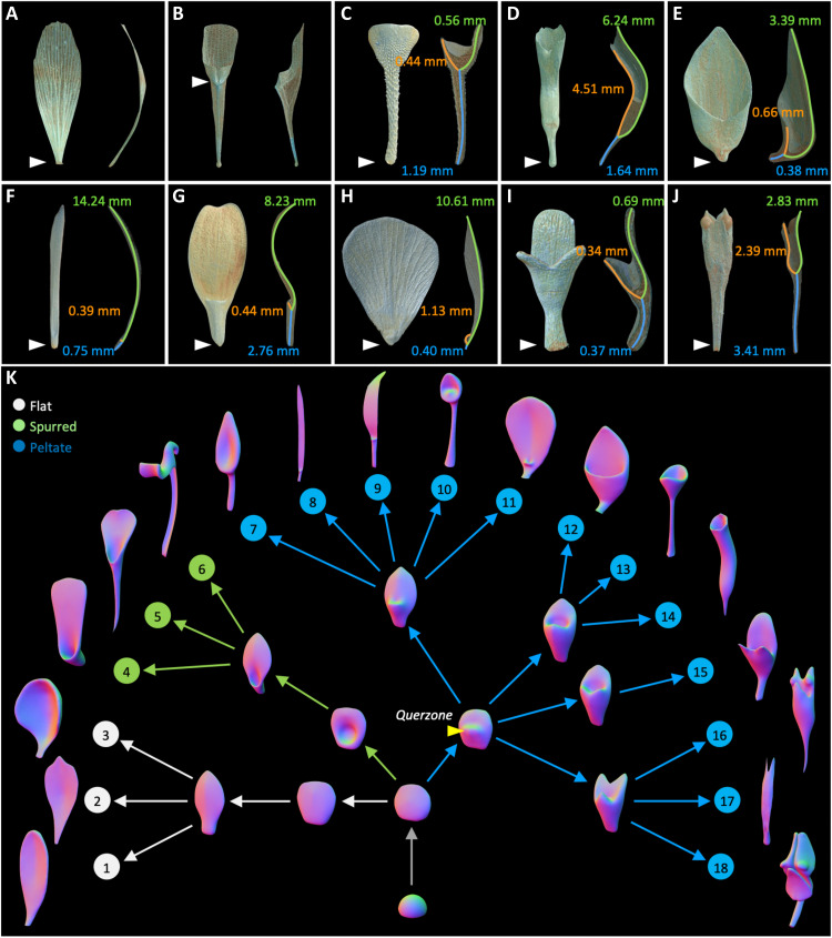
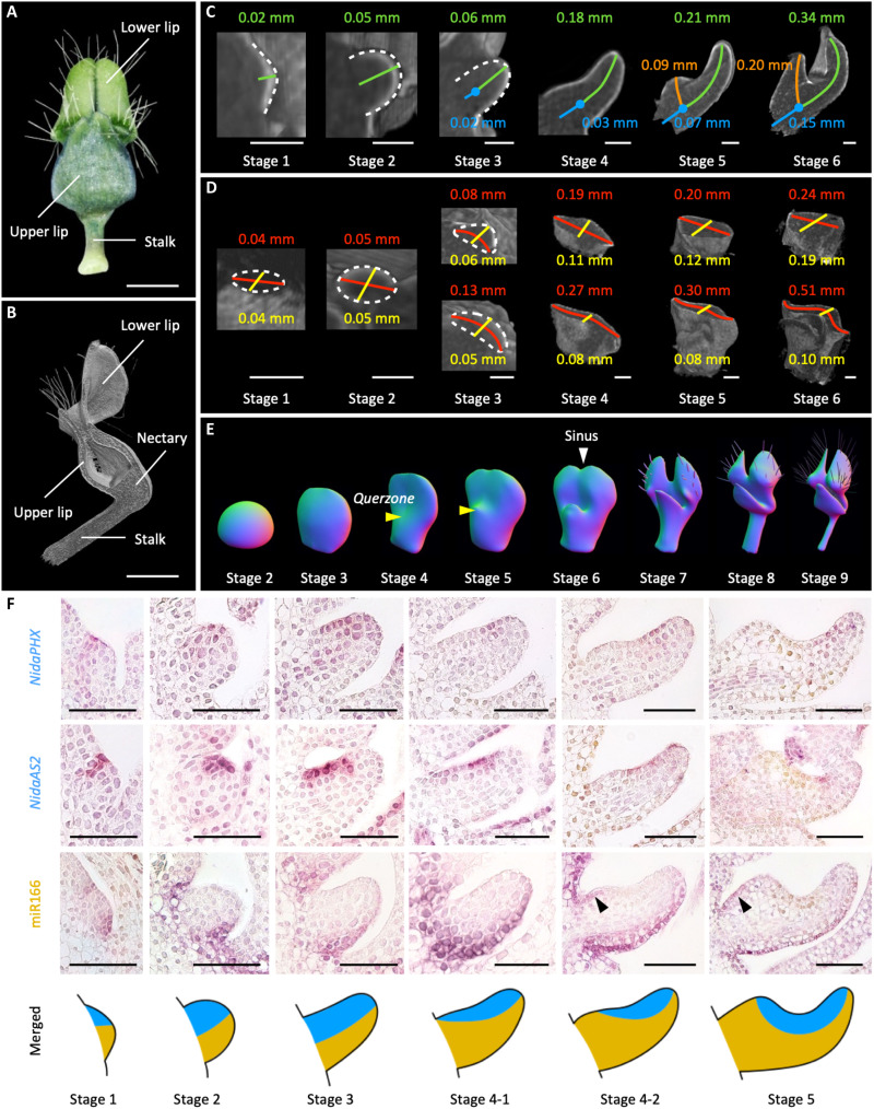
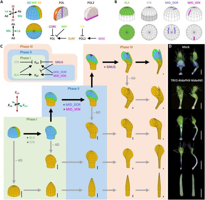
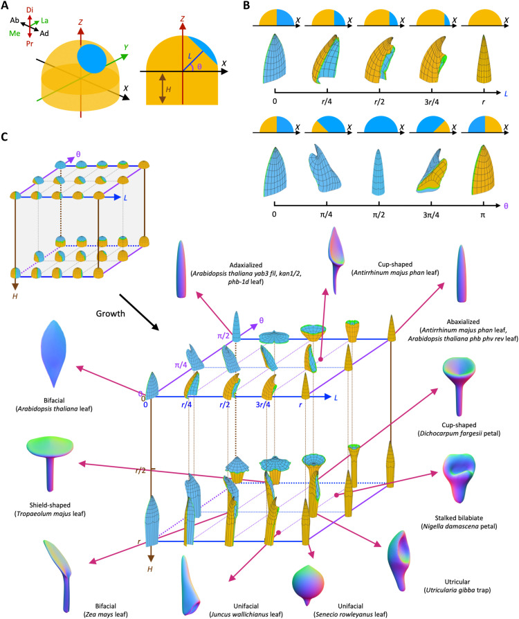
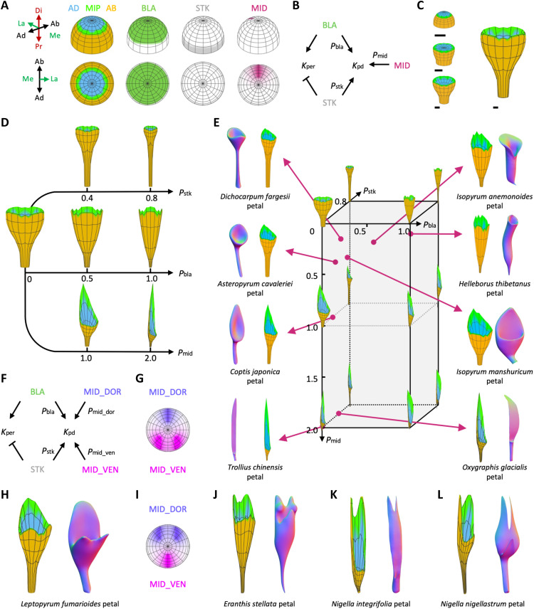
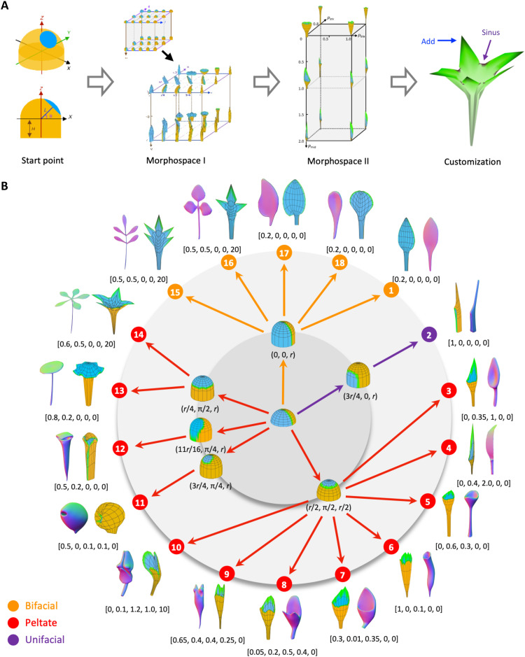
Peltate organs, such as the prey-capturing traps of carnivorous plants and nectary-bearing petals of ranunculaceous species, are widespread in nature and have intrigued and perplexed scientists for centuries. Shifts in the expression domains of adaxial/abaxial genes have been shown to control leaf peltation in some carnivorous plants, yet the mechanisms underlying the generation of other peltate organs remain unclear. Here, we show that formation of various peltate ranunculaceous petals was also caused by shifts in the expression domains of adaxial/abaxial genes, followed by differentiated regional growth sculpting the margins and/or other parts of the organs. By inducing parameters to specify the time, position, and degree of the shifts and growth, we further propose a generalized modeling system, through which various unifacial, bifacial, and peltate organs can be simulated. These results demonstrate the existence of a hierarchical morphospace system and pave the way to understand the mechanisms underlying plant organ diversification.

Fig. 1.. Structures and diversification of ranunculaceous petals.

(A to J) Front views and longitudinal sections [in micro–computed tomography (micro-CT)] showing the petals of 10 representative species: Adonis sutchuenensis (A), Aquilegia viridiflora (B), Dichocarpum fargesii (C), Helleborus thibetanus (D), Isopyrum manshuricum (E), Trollius chinensis (F), Oxygraphis glacialis (G), Ranunculus japonicus (H), Leptopyrum fumarioides (I), and Eranthis stellata (J). Green, blue, and orange lines mark the lengths of the lower lip, stalk, and upper lip, respectively, whereas white arrowheads mark the attached points of the petals on the receptacles. Measurements are given in the same colors as the lines. (K) Virtual clay models showing the trajectories of petal development in A. sutchuenensis (1), Actaea asiatica (2), Anemonopsis macrophylla (3), Urophysa rockii (4), A. viridiflora (5), Aconitum kusnezoffii (6), Coptis japonica (7), T. chinensis (8), O. glacialis (9), Asteropyrum cavaleriei (10), R. japonicus (11), I. manshuricum (12), D. fargesii (13), H. thibetanus (14), L. fumarioides (15), E. stellata (16), N. integrifolia (17), and N. damascena (18), as described (4, 5, 21, 22). Yellow arrowhead points to the Querzone.

Fig. 2.. Development of Nigella damascena petals and expression of key adaxial and abaxial genes.

(A and B) Front view (A) and longitudinal section [(B); in micro-CT] of a mature petal of N. damascena, with the lower lip, upper lip, stalk, and nectary being marked. (C and D) Longitudinal (C) and transverse (D) sections (in micro-CT) of the petals at different developmental stages (1 to 6). In (C), green, blue, and orange lines mark the lengths of the lower lip, stalk, and upper lip, respectively. In (D), red lines mark the widths of the primordia (stages 1 and 2), the lower lips (the bottom row from stages 3 to 6), and the stalks (the top row from stages 3 to 6); yellow lines mark the thicknesses of the primordia (stages 1 and 2), the lower lips (the bottom row from stages 3 to 6), and the stalks (the top row from stages 3 to 6); white dotted lines mark the outlines of longitudinal and transverse sections of the primordia. Measurements are given in the same colors as the lines. (E) Successive virtual clay models showing the development of the N. damascena petals, with yellow arrowheads pointing to the Querzone and white arrowhead pointing to the sinus. (F) Expression patterns of NidaPHX, NidaAS2, and miR166 during petal development, with black arrowheads indicating the positions of the ectopic expression. In the merged diagram, the blue and brown areas represent the adaxial and abaxial domains, respectively. Scale bars, 100 μm in (A) and (B) and 50 μm in (C), (D), and (F).

Fig. 3.. Simulation of N. damascena petals and functional verification.

(A and B) Initial setups of the model. Oblique and top views show the distributions of the factors used (i.e., AD, AB, MIP, BLA, STK, MID_DOR, and MID_VEN). Ad, adaxial; Ab, abaxial; Pr, proximal; Di, distal; Me, medial; La, lateral. POL (black arrows) runs from SURF toward MIP and CORE, whereas POL2 (red arrows) runs from BASE to the TIP. (C) Modeling process and the results. Patterns of growth in different phases (phases I to III) are determined by different growth rate regulatory networks: BLA and STK regulate the differential growth in phase I; MID_DOR and MID_VEN promote the expansion of local areas in phase II; and SINUS inhibits the local growth in phase III. Different final states are obtained when AD is removed from the beginning of different developmental phases. (D) Petals of the mock and those of TRV2-NidaPHX-NidaANS–treated plants with strong phenotypic changes. Scale bars, 100 μm.

Fig. 4.. A simple and generalized modeling system for simulating various basic shapes.

(A) Schematic diagrams (oblique and sagittal section views) showing the parameters of the initial model. L refers to the distance between the original point (0, 0, 0) of the coordinate system and the midplane of AD and AB domains, θ refers to the angle between the normal of the midplane and X-Y plane (Z = 0), and H refers to the height of the cylindrical base. (B) Initial (section view) and final states (oblique view) of the models by increasing the values of parameter L (from 0 to r) or θ (from 0 to π). r is the radius of the hemispheric tip of the primordium. (C) Three-dimensional morphospaces showing the initial and final states of the models by changing the values of L (from 0 to r), θ (from 0 to π/2), and H (from 0 to r). Representative organs resembling the corresponding shapes are presented with virtual clay models.

Fig. 5.. Simulation of the diverse peltate petals within the Ranunculaceae.

(A) Oblique and top views showing the distributions of the factors used (i.e., AD, AB, MIP, BLA, STK, and MID). (B) Growth rate regulatory network (KRN) of the model. (C) Developmental stages of the model when P_stk = 0, P_bla = 0, and P_mid = 0. Scale bars are in arbitrary units. (D) Final states of the models by changing the values of P_stk (0.4, 0.8), P_bla (0.5, 1.0), and P_mid (1.0, 2.0), respectively. (E) Resultant morphospace showing the final states of the models. Representatives of different subtypes of peltate petals are presented with virtual clay models. (F to L) Models of peltate petals with marginal elaborations. In the modified KRN, MID is replaced by MID_DOR and MID_VEN (F). Distributions of MID_DOR and MID_VEN (top view) are shown in (G) and (I), and the final states of the models, which correspond to the petals of four ranunculaceous species, are shown in (H) and (J) to (L).

Fig. 6.. Generation of diverse plant lateral organs with a generalized modeling system.

(A) Hierarchical nature of the modeling system. (B) Modeling of plant lateral organs with various basic shapes and marginal modifications within the generalized modeling system. The inner circle shows the changes from a start point (i.e., a hemispheric bifacial primordium) to various intermediate states by adjusting the values of L, θ, and H (in round brackets). The outer circle shows the changes from various intermediate states to more final states by adjusting the values of P_bla, P_stk, P_{mid_dor}, P_{mid_ven}, and P_sinus (in square brackets). Real examples of the final states include the following: the simple bifacial leaf of A. thaliana (1); the unifacial leaf of J. wallichianus (2); the peltate petals of C. japonica (3), O. glacialis (4), D. fargesii (5), H. thibetanus (6), I. manshuricum (7), L. fumarioides (8), E. stellata (9), and N. damascena (10); the utricular traps of U. gibba (11); the pitcher-shaped leaf of Sarracenia flava (12); the shield-shaped leaf of T. majus (13); the peltately palmate compound leaf (14); the pinnate compound leaf (15); the ternately compound leaf (16); the asymmetrical leaf (17); and the simple petal (18).

References

1. D. Franck, The morphological interpretation of epiascidiate leaves—An historical perspective. Bot. Rev. 42, 345–388 (1976).
1. W. Troll, Morphologie der schieldförmigen blätter. Planta 17, 153–230 (1932).
1. C. Thorogood, U. Bauer, S. Hiscock, Convergent and divergent evolution in carnivorous pitcher plant traps. New Phytol. 217, 1035–1041 (2018). - PubMed
1. C. Erbar, S. Kusma, P. Leins, Development and interpretation of nectary organs in Ranunculaceae. Flora 194, 317–332 (1999).
1. K. Kosuge, Petal evolution in Ranunculaceae. Plant Syst. Evol. 8, 185–191 (1994).