Bioinspired figure-ground discrimination via visual motion smoothing

Abstract

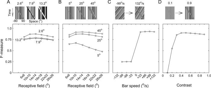
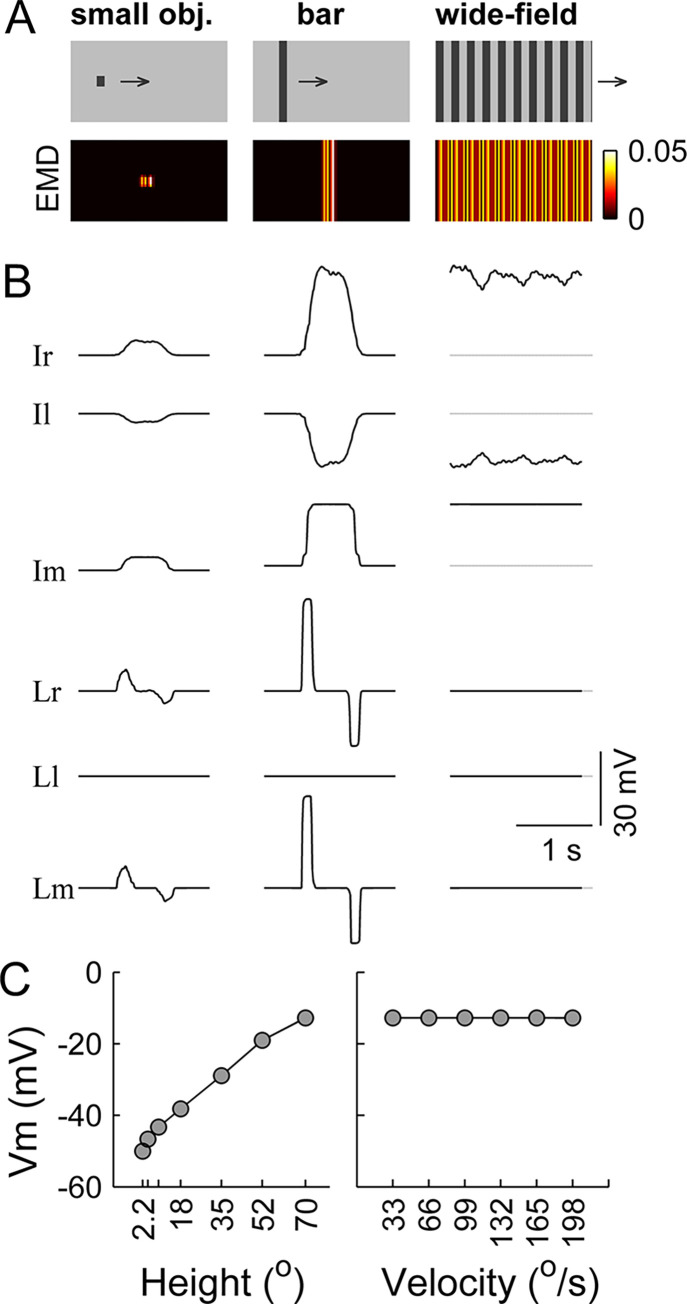
Flies detect and track moving targets among visual clutter, and this process mainly relies on visual motion. Visual motion is analyzed or computed with the pathway from the retina to T4/T5 cells. The computation of local directional motion was formulated as an elementary movement detector (EMD) model more than half a century ago. Solving target detection or figure-ground discrimination problems can be equivalent to extracting boundaries between a target and the background based on the motion discontinuities in the output of a retinotopic array of EMDs. Individual EMDs cannot measure true velocities, however, due to their sensitivity to pattern properties such as luminance contrast and spatial frequency content. It remains unclear how local directional motion signals are further integrated to enable figure-ground discrimination. Here, we present a computational model inspired by fly motion vision. Simulations suggest that the heavily fluctuating output of an EMD array is naturally surmounted by a lobula network, which is hypothesized to be downstream of the local motion detectors and have parallel pathways with distinct directional selectivity. The lobula network carries out a spatiotemporal smoothing operation for visual motion, especially across time, enabling the segmentation of moving figures from the background. The model qualitatively reproduces experimental observations in the visually evoked response characteristics of one type of lobula columnar (LC) cell. The model is further shown to be robust to natural scene variability. Our results suggest that the lobula is involved in local motion-based target detection.

Fig 1. Schematic diagrams of the model.

(A) EMD-lobula network. Individual EMD units comprise parallel ON and OFF pathways, which are exactly the same as shown in Fig 4A in the paper by Eichner et al. [39]. The output of the ON+OFF EMD array, as a retinotopic summation of two EMD arrays in the ON and OFF pathways, is projected to the Ir and Il modules. The outputs of Ir and Il are retinotopically added and projected to the Im module. The Lr, Ll, and Lm modules are postsynaptic to Ir, Il, and Im, respectively. Six lobular modules share the same array size as that of the ON+OFF EMD array. (B) Structures of example receptive fields of units belonging to Il (left panel in B1); Ir (right panel in B1); Im (B2); and Lr, Ll, and Lm (B3). Δϕ is the spatial interval between adjacent presynaptic units.

Fig 2. The lobula network solves figure-ground discrimination problems based on the noisy local motion measured by an EMD array.

(A) One example of an input frame. The stimulus (80% contrast) consisted of a textured foreground figure (34° × 34°, in the red boundary) moving to the right at a speed of 66°/sec against a similarly textured background (stationary) (S1 Video). The red boundary was not present in the actual stimuli. Left: the original frame. Middle: the preprocessed image. Right: the foreground location (white area) and the background (black area). (B) Snapshot of the response profile of the ON+OFF EMD array. To examine the profile (top) at a higher resolution, the area outlined by the cyan boundary was zoomed in and disassembled into rightward (lower-right) and leftward (lower-left) components. (C) Same as (B) except that the EMD response profiles in the ON and OFF pathways were also displayed (upper row). All data were displayed as a grayscale matrix. The area in each panel outlined by the white boundary was magnified and disassembled into rightward (lower-right) and leftward (lower-left) components. Note: the element values were enlarged by 10-fold in the lower panels to facilitate an inspection of the difference between the numbers of elements of two components. (D) Foreground figures detected in the Ir module under different receptive field conditions (labeled at the top). Upper row: membrane potentials of the units in the Ir module. Lower row: output of the Ir module. Red boundaries indicate the figure’s locations at the corresponding instant in time. The membrane potential time courses of five units (marked by white circles) were further examined under two receptive field conditions in (F). (E) Membrane potentials of the units in the Lr module (simultaneously recorded with those in (D)). (F) Time courses of the membrane potentials of the five units marked in (D). The curves are color-coded according to the marking colors of the corresponding units in (D). The data in (A-E) are presented based on the input frame in (A). The synaptic weights of the projections between lobula modules were set as α^lo→lo = 2.

Fig 3. Individual lobula modules extract stimulus features depending on their receptive field structures and direction selectivity.

Data are presented vertically according to their stimulus classes (indicated at the top) and shown based on the input frame at which the foreground figure passed the middle of the visual field. The receptive field of the units in Ir and Il on the EMD array was set as 26° × 26°. (A) Space-time plots of three classes of stimuli with a contrast level of 80% and a moving speed of 66°/sec. Each plot illustrates how the top row (horizontal axis) evolved with time (vertical axis). The top row was randomly selected from the rows of the first frame of stimulus images, so the row evolution characterizes the dynamic evolution of the stimulus. In ‘Bar on Ground’, the background was moving in the direction opposite of the bar (25° × 90°) at the same speed. In ‘Theta Figure’, the elements within the bar (25° × 90°) moved to the left, and the bar itself moved to the right at the same speed. (B) Output of the ON+OFF EMD array (upper row). The area outlined by the white boundary in each panel was magnified and disassembled into rightward (lower-right) and leftward (lower-left) motion components. The element values were enlarged by 10-fold in the lower panels to facilitate an inspection of the difference between the numbers of elements of the two components. (C) Membrane potentials (upper row) and corresponding outputs (lower row) of the units in the Ir, Il, and Im modules. Red boundaries indicate the actual locations of the moving foregrounds at the corresponding instant in time. The membrane potential time courses of the units (marked by white circles) were further examined in (E). (D) Membrane potentials of the units in the Lr, Ll, and Lm modules (simultaneously recorded with those in (C)). (E) Time courses of the membrane potentials of the units marked in (C). The curves are color-coded according to the marking colors of the corresponding units in (C).

Fig 4. Dissecting the figure-ground discrimination process in the pathway from the EMD array to the Ir module.

(A) Snapshots of the segmented foreground (white area) and background (black area) at three stages: the output of the EMD array (left column), the input of the Ir module (middle column), and the output of the Ir module (right column). The segmentation threshold was set as 50% maximum (top row) or 10%, 30%, 70%, and 90% maximum (bottom row). The stimulus was a textured 25° bar (80% contrast), which was moving against a similarly textured background at 66°/sec (upper leftmost: space-time plot). Data are presented based on the input frame at which the bar passed the middle of the visual field. (B) Instantaneous F-measure throughout the entire stimulus presentation period. It was evaluated by using a segmentation threshold of 50% maximum at three stages: the output of the EMD array (green curve), the input of the Ir module (light blue curve), and the output of the Ir module (dark blue curve). (C) and (D) are the same as (A) and (B), respectively, except that the stimulus background was moving in the direction opposite of the bar. For all simulations, the receptive field of the units in Ir and Il on the EMD array was set as 10°×10°.

Fig 5. Effect of the membrane time constant τ_m on figure-ground discrimination.

(A) Figure-ground segmentation effect achieved with the same stimulus as that used in Fig 4A. Leftmost panel: space-time plot of the stimulus. The 1st to 3rd rows: snapshots of the segmented foreground (white area) and background (black area) at three stages (the output of the EMD array (1st row), the input of the Ir module (2nd row), and the output of the Ir module (3rd row)). The snapshots are presented based on the input frame at which the bar passed the middle of the visual field. The segmentation threshold was set as 50% maximum. The corresponding τ_m value is indicated at the top. The 4th row: instantaneous F-measures throughout the entire stimulus process evaluated at the output of the EMD array (green curve), the input of the Ir module (light blue curve), and the output of the Ir module (dark blue curve). (B1) Same as (A), except the stimulus was replaced by ‘Theta Figure in Moving Background’ (leftmost panel). The stimulus featured a background moving to the left at 66°/sec. The bar shared exactly the same motion as the background, whereas the elements within the bar coherently moved to the right at 66°/sec. (B2) Same as (B1), except the dot size of the stimulus was changed from 2.6° to 7.9°.

Fig 6. Effects of the receptive field size and stimulus parameters on figure-ground discrimination.

Unless specified below, the receptive field size of the lobula units on the EMD array was set as 14° × 14°, and a moving bar (25° width; 80% contrast; 2.6° dot resolution; 66°/sec speed) with a stationary background was used as the stimulus. The F-measures were averaged across the input frames (with the initial 50 frames excluded as transient frames) at the output stage of the Ir module. (A-B) Effect of the receptive field size on the averaged F-measure under different stimulus conditions. In panel (A), three dot resolutions, as specified at the top of each space-time plot, were tested: 2.6° (squares), 7.9° (triangles), and 13.2° (circles). In panel (B), three bar widths, as specified at the top, were tested: 5° (triangles), 25° (squares), and 45° (circles). (C-D) Effects of the stimulus velocity (C) and contrast (D) on the averaged F-measure. In panel (C), the background was not stationary but rather moving at −132°/sec, and the bar’s velocity was varied as specified along the abscissa axis.

Fig 7. Stimulus-evoked responses at the single-unit level in the lobula network.

(A) Three classes of stimuli (upper row, with their names indicated) and the corresponding output of the ON+OFF EMD array (lower row). The ‘small obj.’ and the ‘bar’ had figures with sizes of 8.9° × 8.9° and 8.9° × 70°, respectively, and the luminance levels of their foreground and background were set as 0.25 and 0.75, respectively. The ‘wide-field’ square grating had a spatial wavelength of 17.8° and a Michelson contrast of 50%, and its luminance was periodically set as 0.25 and 0.75. All the stimuli had 70° x 180° visual fields and moved rightward at 33°/sec. (B) Stimulus-evoked membrane potentials in the six lobula modules with the names indicated beside each row. Only the response of the centrally located unit in each module is displayed. Dashed lines indicate the resting membrane potentials. (C) Effects of the bar height and speed on the depolarization extent of the Lm module. Only the data of the centrally located unit are displayed. Left panel: the peak of the evoked membrane potential versus the bar height. Right panel: the peak of the evoked membrane potential versus the bar speed. For all simulations, the synaptic weights of the projections from the EMD array to the postsynaptic lobula modules were set as α^EMD→lo = 100.

Fig 8. Effect of simulated octopaminergic modulation on the lobula network.

(A) Two classes of stimuli. The dark bar (0 luminance; 8.9° width) moved rightward at a speed of 33°/sec over a background square grating with a Michelson contrast of 33% (the luminance was periodically set as 0.25 and 0.5; 17.8° spatial wavelength). The grating was either stationary (the ‘bar’ stimulus) or moving with the same velocity as the bar (the ‘bar+bg’ stimulus). The visual field was 70° × 180°. (B) Stimulus-evoked membrane potentials with (red curves) and without (black curves) octopaminergic modulation in the six lobula modules with the names indicated beside each row. Only the responses of the centrally located unit in each module were displayed. Octopaminergic modulation was realized by changing the half-activation voltage θ of the activation function of the Ir and Il modules from −40 mV to −28 mV. Dashed lines indicate the resting membrane potentials. (C) F-measure obtained under the corresponding stimulus condition. The F-measure with (red curves) and without (black curves) octopaminergic modulation was evaluated at the output stage of the Ir module during the continuous presentation of 300 input frames. For all simulations, the synaptic weights of the projections from the EMD array to the postsynaptic lobula modules were set as α^EMD→lo = 100.

Fig 9. Effect of the modulated half-activation voltage on the responses of the units in the Lm module.

(A) Same stimulus as ‘bar’ in Fig 8A. (B) Same data as shown in the panel located in the bottom row and the 1st column of Fig 8B. (C) Stimulus-evoked membrane potentials in Lm (2nd to 7th columns). Only the responses of the centrally located unit in Lm are displayed. By shifting the half-activation voltage θ to less negative values (indicated on the top of each column), the sigmoid function (black curves, 1st column) was shifted to the right (pink and red curves, 1st column). The module names to which the mimicked octopamine modulation process was applied are marked on the top of the 1st column. (D) Same stimulus as ‘bar+bg’ in Fig 8A. (E) Same data as shown in the panel located in the bottom row and the 3rd column of Fig 8B. (F) Same as (C) except that the simulation was performed with the ‘bar+bg’ stimulus in (D). The scale bars in the bottom right corner apply to all the membrane potentials. Except for θ, all parameter values were the same as those used to produce the results shown in Fig 8.

Fig 10. Effect of the modulated steepness on the responses of the units in the Lm module.

(A) and (B) are the same as Fig 9A and 9B, respectively. (C) Stimulus-evoked membrane potentials in Lm (2nd to 7th columns). Only the responses of the centrally located unit in Lm are displayed. The parameter β was set as indicated on the top of each column, accordingly changing the sigmoid function’s steepness (4 curves in the 1st column). The half-activation voltage θ was fixed at –40 mV (upper row) or –28 mV (lower row). The scope of parameter modulation covered the Ir, Il, and Im modules. (D) and (E) are the same as Fig 9D and 9E, respectively. (F) Same as (C) except that the simulation was performed with the ‘bar+bg’ stimulus in (D). The scale bars in the bottom right corner apply to all the membrane potentials. Except for β and θ, all parameter values were the same as those used to produce the results shown in Fig 8.

Fig 11. Figure-ground discrimination results produced by the model in the case of cluttered natural scenes.

(A) Schematic illustration of the synthesized stimuli covering a full 360° azimuth and a 97° elevation. The foreground was a gray bar with a width of 15° and 0.5 luminance intensity, as illustrated in the panel located in the 1st row and 1st column, in which the arrowhead and three arrows express the movement directions of the bar and the background, respectively. The image background moving in reverse shared the same speed with the bar. The C_RMS levels of the images in the 1st column from top to bottom are 5.74, 3.89, 2.10, 1.59, and 1.28, respectively. The C_RMS levels of the images in the 2nd column from top to bottom are 1.19, 0.92, 0.88, 0.69, and 0.43, respectively. (B) F-measures evaluated at three stages along the pathway from the EMD array to the Il module: the output of the EMD array (green curve), the input of Il (light blue curve), and the output of Il (dark blue curve and black curve). The F-measures were averaged across all 10 conditions of the background scene for each stimulus speed. Error bars indicate the standard deviations. The synaptic weights of the projections from the EMD array to the postsynaptic units were set as α^EMD→lo = 100 (all curves except the black one) and 200 (the black curve), respectively.

References

1. Bishop LG, Keehn DG. Neural correlates of the optomotor response in the fly. Kybernetik. 1967; 3:288–295. doi: 10.1007/BF00271512 - DOI - PubMed
1. Bishop LG, Keehn DG, McCann GD. Motion detection by interneurons of optic lobes and brain of the flies Calliphora phaenicia and Musca domestica. J Neurophysiol. 1968; 31:509–525. doi: 10.1152/jn.1968.31.4.509 - DOI - PubMed
1. Dvorak DR, Bishop LG, Eckert HE. On the identification of movement detectors in the fly optic lobe. J comp Physiol. 1975; 100:5–23. 10.1007/BF00623928 - DOI
1. Hausen K. Functional characterization and anatomical identification of motion sensitive neurons in the lobula plate of the blowfly Calliphora erythrocephala. Z Naturforsch. 1976; 31c:629–633.
1. Borst A, Haag J, Reiff DF. Fly Motion Vision. Annu Rev Neurosci. 2010; 33:49–70. doi: 10.1146/annurev-neuro-060909-153155 - DOI - PubMed
Publication types