The nematode worm C. elegans chooses between bacterial foods as if maximizing economic utility

Abstract

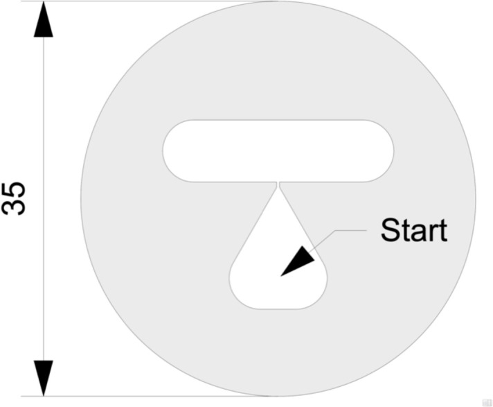
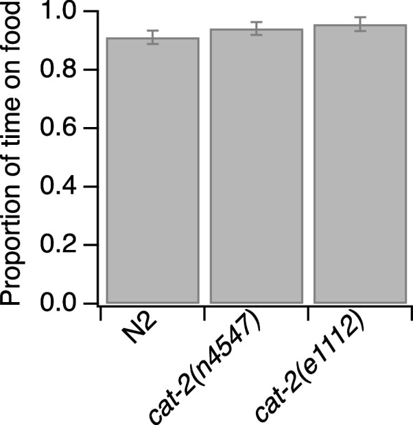
In value-based decision making, options are selected according to subjective values assigned by the individual to available goods and actions. Despite the importance of this faculty of the mind, the neural mechanisms of value assignments, and how choices are directed by them, remain obscure. To investigate this problem, we used a classic measure of utility maximization, the Generalized Axiom of Revealed Preference, to quantify internal consistency of food preferences in Caenorhabditis elegans, a nematode worm with a nervous system of only 302 neurons. Using a novel combination of microfluidics and electrophysiology, we found that C. elegans food choices fulfill the necessary and sufficient conditions for utility maximization, indicating that nematodes behave as if they maintain, and attempt to maximize, an underlying representation of subjective value. Food choices are well-fit by a utility function widely used to model human consumers. Moreover, as in many other animals, subjective values in C. elegans are learned, a process we find requires intact dopamine signaling. Differential responses of identified chemosensory neurons to foods with distinct growth potentials are amplified by prior consumption of these foods, suggesting that these neurons may be part of a value-assignment system. The demonstration of utility maximization in an organism with a very small nervous system sets a new lower bound on the computational requirements for utility maximization and offers the prospect of an essentially complete explanation of value-based decision making at single neuron resolution in this organism.

Keywords: C. elegans; chemosensation; decision making; foraging behavior; neuroeconomics; neuroscience; subjective value; transitivity.

Figure 1.. Design of a GARP experiment and tests for utility maximization.

(A) Direct violation of utility maximization. Diagonal lines indicate choice sets ($n$=11). Choice sets are distinguished by having different values of the overall budget and/or different prices for at least one of the goods. Within a choice set, the expenditure implied by each bundle of goods is constant and equals the budget. In A (blue), the budget is $8, oranges are $2 per unit, apples are $1 per unit. In B (red): the budget is $8, oranges are $1 per unit, apples are $2 per unit. Filled circles, chosen amounts; plus signs, available amounts not chosen. Given the choices shown and the more is better rule, $a\succcurlyeq d\succ b⟹a\succ b$ and $b\succcurlyeq c\succ a⟹b\succ a$. Therefore, choices $a$ and $b$ directly violate utility maximization. (B). Indirect violation of utility maximization. Symbols as in A. The choices $a$ and $c$ constitute an indirect violation of utility maximization as described in the text.

Figure 2.. Edible bacteria act as goods over which worms form preferences through experience.

(A) Food quality training and preference assays. Filled circles represent patches of bacteria as indicated in the key. Stars indicate worm starting locations. (B). Mean preference at $t=$ 60 min. in the open-field accumulation assay for trained and untrained N2 and ceh-36 mutants. Asterisk, see Table 2¹. Replicates, Trained, strain($N$): N2(8), ceh-36(9). Replicates, Untrained, strain($N$): N2(8), ceh-36(8). (C). Mean preference vs. time for trained and untrained N2 worms in T-maze accumulation assays, with and without sodium azide in the food patches. (D). Mean preference index vs. time for trained and untrained cat-2(tm2261) mutants and N2 controls in T-maze accumulation assays. N2 data are from C. (B–D). Error bars, 95% CI. For sample size (N), statistical methods used, and significance level, see Table 2, rows 1-15.

Figure 2—figure supplement 1.. T-maze diagram.

The teardrop shaped feature acts as worm diode. Worms leave the teardrop more easily than they re-enter it, thus helping to ensure they do not congregate at the starting point. The mask’s ability to confine worms in the test area is improved by floating the maze on the surface of the agarose medium while it is still liquid (M. Brooks, pers. comm.). Dimensions are in mm.

Figure 2—figure supplement 2.. Loss of dopamine signaling does not reduce proportion of time on food.

Mutations in the gene cat-2 do not significantly later the ability of worms to find and remain in food patches. Statistics (t-tests): N2 vs. cat-2(n4547), t(38) = –0.95, p=0.35; N2 vs cat-2(e1112), t(40) = –1.38, p=0.18. N2, n = 30; cat-2(n4547), n = 10; cat-2(e1112) n = 12. Error bars, SEM.

Figure 3.. Single-worm food choice assays.

(A) Layout of the Y-chip. Asterisks indicate the position of recording electrodes. Ground electrodes (not shown) were inserted into the food and buffer ports to reduce electrical interference. The chip is shown configured for the experiments in Figures 4B and 5B. (B). Area of detail shown in A. The dashed line is the centerline of chip; the white line within the worm is its centerline. The black arrow connects the middle of the neck where it enters the food channel with anterior end of worm’s centerline. Positive values of head angle ($\theta$) indicate displacement toward H food. Colored arrows show direction of flow. (C). Schematic overview of fluidic system. (D). Typical electropharyngeogram. Each pair of excitation (E) and relaxation (R) spikes constitutes one pharyngeal pump.

Figure 4.. Validation of the Y-chip for measuring food preferences.

(A) Familiar food effect. Mean pump frequency of worms grown on H or M food and tested on the same or the converse food. Asterisk, see Table 2¹⁷. Both foods were at OD 1. Pumping was recorded for 12 min. Replicates, Grown on H, tested on ($N$): Familiar(16), Unfamiliar(6). Replicates, Grown on M, tested on($N$): Familiar(23), Unfamiliar(13). Error bars, 95% CI. (B). Food quality learning. Mean fraction of pumps in H food in trained and untrained worms. Asterisk, see Table 2²⁰. The dashed line indicates equal preference for H and M food. Both foods were at OD 1. Error bars, 95% CI. (C,D). Time course of pump frequency at four different densities of familiar food. Food enters the chip at $t=0$ sec. Optical density is indicated next to each trace. The black trace shows pumping in the absence of food. Shading, ± SEM E. Dependence of mean peak pump frequency density of familiar food. (F). Dependence of latency to half-maximal pump frequency on density of familiar food. (E,F). Error bars, 95% CI. For sample size (N), statistical methods used, and significance level, see Table 2, rows 16-000.

Figure 5.. Economic analysis of food choice in C. elegans.

(A) Demand curves. Mean consumption of familiar food versus its price. Consumption is computed as number of pumps times optical density of bacteria. Price is computed by Equation 2. The data are fit by Equation 8 with $ϵ=-2.2$ for H food and $ϵ=-1.9$ for M food. H food price($N$): 0.33(13), 1.0 (16), 3.3 (21), 10(15). M food price($N$): 0.33(9), 1.0 (23), 3.3 (7), 10(10). (B). Price ratio curves. Food preference, measured as fraction of pumps in H food, versus price ratio for Trained and Untrained worms. Horizontal dashed line: indifference between H and M food; vertical dashed line: H and M food at equal price. Data at log price ratio = 0 are replotted from Figure 4B. Replicates, Trained, point($N$): a(9), b(14), c(18), d(27), e(20), f(10), g(6). Replicates, Untrained, point($N$): a(12), b(17), c(13), d(12), e(28), f(10), g(7). (C). GARP analysis of C. elegans food preferences. Plotted points show mean consumption of M food versus consumption of H food in Trained and Untrained worms. Lines are choice sets as in Figure 1. The $x$ and $y$ intercepts of each line indicate the amounts of H and M food that would have been consumed if the worm spent all its pumps on one or the other food type. Error bars, 95% CI. (D). Predicted consumption of H and M food in Trained and Untrained animals on a widely-used ensemble containing 11 budget lines (Harbaugh et al., 2001). (A–C). Error bars, 95% CI. For sample size (N), statistical methods used, and significance level, see Table 2, rows 23-26.

Figure 5—figure supplement 1.. Distributions of preference values in trained and untrained animals in Figure 5B.

Figure 5—figure supplement 2.. Indirectly revealed preferences inherent in the choices shown in Figure 5C.

Figure 6.. Higher order features of utility maximization.

(A) H and M food act as substitutes. Consumption is plotted against price for triplets of cost ratios in which the concentration of one food was constant and the concentration of the other food was variable (see Supplementary file 1). Lower case italic letters: data points in Figure 5B. Capital letters: the food whose density was constant, the consumption of which is plotted on the $y$-axis. Solid lines: regression slope different from zero ($p\le 0.01$); dashed lines: slope not different from zero. Error bars, 95% CI. (B). H and M food are not perfect substitutes. Colored contour lines are indifference curves in a perfect substitute model (Equation 10) with $\beta =10/11$. Data points from Figure 5C are replotted for comparison, with associated budget lines, according to the conventions of that figure. ‘X’ symbols indicate the point of highest utility on each budget line. (C–D). Best fitting parameterizations of the CES function (Equation 11) for Trained and Untrained animals. Each panel shows the seven the iso-utility lines that are tangent to the budget lines. Goodness of fit can be assessed by observing that the iso-utility lines are tangent to the budget lines at, or near, the data points which indicate mean consumption of H and M food. For sample size (N), statistical methods used, and significance level, see Table 2, rows 27-32.

Figure 7.. Behavioral mechanisms of utility maximization.

(A) Pumping-rate model of preference. Equation 13 is evaluated for each worm in Figure 5B and the result is plotted against preference in terms of fraction of pumps in H food for the same animal. (B). Dwell-time model of preference. Same as A but using Equation 14. (C). Regression of Equation 14 against mean head angle as defined in Figure 3B. (A–C). Blue lines: regressions on the data. (D). Diminished ceh-36 function eliminates the effect of food quality training on food preference. Asterisk, see Table 2³⁸. (H and M) are at OD = 1. N2 data are from Figure 4B. Replicates, Trained, strain($N$): N2(20), ceh-36(7). Replicates, Untrained, strain($N$): N2(28), ceh-36(11). Error bars, 95% CI. Correlation coefficients are shown ±95% CI. For sample size (N), statistical methods used, and significance level, see Table 2, rows 33-39.

Figure 8.. Characterization of AWC’s response to delivery and removal of food.

(A) Ensemble averages of relative fluorescence versus time in response to onset of the indicated food in trained and untrained animals. (B). Summary of data in A, showing mean integrated calcium transients. (C). Ensemble averages of relative fluorescence versus time in response to removal of the indicated food in trained and untrained animals. Asterisk: untrained group, mean peak response, H vs. M food, see Table 2⁴². Cross: trained group, mean peak response, H vs. M food, see Table 2⁴³. (D). Summary of data in C, showing mean integrated calcium transients Asterisk, see Table 2⁴⁶. (A–D). OD = 1 for H and M food. Shading, ± SEM. Error bars, 95% CI. For sample size (N), statistical methods used, and significance level, see Table 2, rows 40-47.

Figure 8—figure supplement 1.. Imaging chip.

Fluidic features are shown in black. Dimensions are in mm.

Figure 9.. Characterization of AWC’s response to bacterial foods in Y-chip assays.

(A) Ensemble average of relative fluorescence versus time in response to transitions from H to M (H→M) or M to H (M→H) food. Asterisk, see Table 2⁴⁸. Both foods were presented at OD = 1. Food was switched at $t$ = 0. H→M, Trained, $N$ = 16; H→M, Untrained $N$ = 14. M→H, Trained, $N$ = 16; M→H, Untrained, $N$ = 15. Shading,±SEM. (B). Typical fluorescence waveform in response to a series of transitions between H and M food. Notation: $F_0$, baseline fluorescence after sustained exposure to H food (≅ 2 min.); ${\displaystyle F_{\mathrm{M}}}$, maximum H→M fluorescence; ${\displaystyle F_{\mathrm{H}}}$, minimum M→H fluorescence. The box delineates the time period of presumptive steady-state responses over which mean response amplitudes $A_{∆F}$ were computed for each recorded worm. (C–E). $A_{∆F}$ versus utility, preference, and log price ratio. Lines and curves are, respectively, linear and gaussian fits. Italic letters refer to labeled points in Figure 5B. Replicates, Trained, point($N$): a(6), b(10), c(18), d(12), e(19), f(10), g(9). Replicates, Untrained. point($N$): a(8), b(11), c(10), d(8), e(12), f(8), g(10). Error bars, 95% CI. For sample size (N), statistical methods used, and significance level, see Table 2, rows 48-55.

Figure 9—figure supplement 1.. Control for mechanical artifacts in the experiment of Figure 9B assays.

This trace shows a typical AWC fluorescence waveform in response to a series of mock transitions between H and M food in which all syringes in the imaging system contained food-free buffer.

Figure 10.. Price ratio curves and utility maximization.

(A) A pair of intersecting budget lines wherein choices a and b are governed by a price-ratio curve (not shown) that is monotonic-increasing. To support a direct violation of GARP, a must be to the right of the intersection of lines A and B, and b must be to the left of it. However, by price-ratio monotonicity, b must lie to the right of a, for reasons described in the text. This constraint precludes direct violations of GARP. (B). Choice data from a human participant in a GARP experiment (Camille et al., 2011). The data are consistent with utility maximization. Inset, price ratio data inferred from the experiment. Log price ratios for points a-k are calculated as ${\displaystyle log{X}_{\mathrm{Z}}/Y_{\mathrm{Z}}}$, where ${\displaystyle X_{\mathrm{Z}}}$ and ${\displaystyle Y_{\mathrm{Z}}}$ are, respectively, the $x$ and $y$ intercepts of budget line $Z$. The fraction of total budget spent on good X is computed as ${\displaystyle x_{\mathrm{Z}}/X_{\mathrm{Z}}}$, where ${\displaystyle x_{\mathrm{Z}}}$ is the amount of good X chosen on line ${\displaystyle Z}$.

References

1. Addessi E, Mancini A, Crescimbene L, Padoa-Schioppa C, Visalberghi E. Preference transitivity and symbolic representation in capuchin monkeys (Cebus apella) PLOS ONE. 2008;3:e2414. doi: 10.1371/journal.pone.0002414. - DOI - PMC - PubMed
1. Afriat SN. The construction of utility functions from expenditure data. International Economic Review. 1967;8:67. doi: 10.2307/2525382. - DOI
1. Afriat SN. Efficiency estimation of production functions. International Economic Review. 1972;13:568–598. doi: 10.2307/2525845. - DOI
1. Andreoni J, Miller J. Giving according to GARP. Econometrica: Journal of the Econometric Society. 2002;70:737–753. doi: 10.1111/1468-0262.00302. - DOI
1. Arbuthnott D, Fedina TY, Pletcher SD, Promislow DEL. Mate choice in fruit flies is rational and adaptive. Nature Communications. 2017;8:e13953. doi: 10.1038/ncomms13953. - DOI - PMC - PubMed
Publication types