Mice identify subgoal locations through an action-driven mapping process

Abstract

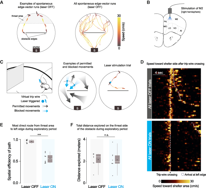
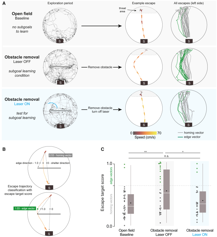
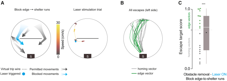
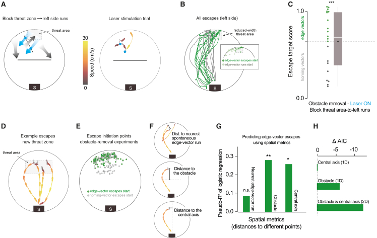
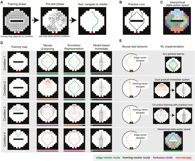
Mammals form mental maps of the environments by exploring their surroundings. Here, we investigate which elements of exploration are important for this process. We studied mouse escape behavior, in which mice are known to memorize subgoal locations-obstacle edges-to execute efficient escape routes to shelter. To test the role of exploratory actions, we developed closed-loop neural-stimulation protocols for interrupting various actions while mice explored. We found that blocking running movements directed at obstacle edges prevented subgoal learning; however, blocking several control movements had no effect. Reinforcement learning simulations and analysis of spatial data show that artificial agents can match these results if they have a region-level spatial representation and explore with object-directed movements. We conclude that mice employ an action-driven process for integrating subgoals into a hierarchical cognitive map. These findings broaden our understanding of the cognitive toolkit that mammals use to acquire spatial knowledge.

Keywords: cognitive map; escape; obstacles; spatial learning; subgoals; threat.

Figure 1

Closed-loop optogenetic activation of M2 interrupts spontaneous edge-vector runs (A) Spontaneous edge-vector runs during the initial exploration period (continuous turn-and-run movements, starting in the threat area and stopping at or moving past the obstacle edge); n = 8 mice. (B) Schematic illustrating optic fiber placement in the right premotor cortex. M2, supplementary motor cortex (premotor cortex); PrL, prelimbic cortex; MO/LO/VO, medial/lateral/ventral orbital cortex; AI, agranular insular cortex. (C) On crossing a virtual trip wire (dashed line) during exploration, mice automatically received a 2-s, 20-Hz light pulse. This caused a stopping and leftward-turning motion preventing the mice from reaching the obstacle edge. In the example trial, the mouse ran to the right side of the platform after the stimulation. Mouse drawing: scidraw.io. (D) All trip-wire crossings, with and without laser stimulation, ordered by time of arrival to the left obstacle edge. Note that mice must be moving toward the shelter area (i.e., southward) to trigger the trip wire. (E) Spatial efficiency is the ratio of the straight-line path to the length of the path taken. White horizontal lines, median; black dots, mean; gray boxes, first and third quartiles; gray vertical lines, range. Each dot represents one mouse/session. p = 5 × 10⁻⁵, one-tailed permutation test. (F) Distance explored on the threat half: p = 0.5, one-tailed permutation test; n = 8 mice in each group.

Figure 2

Interrupting spontaneous edge-vector runs abolishes subgoal learning (A) Black traces show exploration during an example session (open field: 10 min, obstacle removal: 20 min). Lines and silhouette traces show escape routes from threat onset to shelter arrival; open field: 29 escapes; obstacle removal (laser off): 26 escapes; obstacle removal (laser on): 23 escapes. All: n = 8 mice. (B) The initial escape target is the vector from escape initiation to 10 cm in front of the obstacle (black dots), normalized between 0 (shelter direction) and 1 (obstacle edge direction). (C) Escape target scores over 0.65 are classified as edge vectors; scores under 0.65 are classified as homing vectors (as in Shamash et al.²²). Obstacle removal (laser off) vs. open field: p = 0.003; obstacle removal (laser on) vs. open field: p = 0.2; Obstacle removal (laser off) vs. obstacle removal (laser on): p = 0.03, one-tailed permutation tests on proportion of edge-vector escapes.

Figure 3

Blocking edge-to-shelter runs does not diminish subgoal learning (A) Blocking left-edge-to-shelter runs by activating M2 at the obstacle edge. In the example trial, the mouse was stimulated for 10 s and then ran toward the center of the platform. (B) Escapes after obstacle removal. n = 8 mice, 23 escapes (left side). (C) Obstacle removal (block edge-to-shelter) vs. open field: p = 1 × 10⁻⁴; vs. obstacle removal (block edge vectors): p = 0.03; vs. obstacle removal (laser off): p = 0.8; one-tailed permutation tests on proportion of edge-vector escapes.

Figure 4

Subgoal-escape start points are determined by spatial rules (A) Blocking threat-zone-to-left-side runs by changing the trip-wire location and width of the threat zone. In the example trial, there were two consecutive trip-wire crossings (2-s stimulations), after which the mouse moved back toward the threat zone. (B) Escapes after obstacle removal. The reduced-width threat zone ensured that mice would need to cross the deactivated trip wire in order to execute edge-vector escapes; n = 8 mice, 19 escapes (left side). Inset: all start locations for spontaneous edge-vector runs (light green) and subsequent edge-vector escapes (dark green). (C) Obstacle removal (block threat-zone-to-left-side) vs. open field: p = 6 × 10⁻⁴; vs. obstacle removal (block edge vectors): p = 0.01; vs. obstacle removal (laser off): p = 0.8, one-tailed permutation tests on proportion of edge-vector escapes. (D) Four example escapes triggered after obstacle removal with the threat zone in a new position. (E) Pooled data from all obstacle-removal experiments (excepted the block-edge-vectors experiment). Escapes on both the left and right sides are shown. Right-sided escapes are flipped horizontally for visualization, and thus, all the green dots can be seen as left-edge vectors. Each dot represents one escape; n = 40 sessions, 207 escapes. (F) Illustration of three spatial metrics used to predict the likelihood of executing an edge-vector escape. Silhouettes in each arena image are an example escape; orange trajectories in the top image illustrate the corresponding history of edge-vector runs in the exploration period. Black bar shows the distance being measured. (G) McFadden’s pseudo-R² measures the strength of the relationship between each metric and the odds of executing edge-vector escapes. Values of 0.2–0.4 represent “excellent fit.” Distances are measured from the escape initiation point of each escape. For the distance to the nearest spontaneous edge-vector run start point, only runs toward the same side as the escape are considered. Distance to the nearest start point of a spontaneous edge-vector run: pseudo-R² = 0.086; p = 0.5. Distance to the obstacle: pseudo-R² = 0.28; p = 0.007. Distance to the central axis: pseudo-R² = 0.26; p = 0.01. (H) Akaike Information Criterion (AIC) analysis on a logistic regression with different predictors. Decreases in AIC represent better model fit and include a penalty for using additional predictors; ΔAICi = AICi – AICmin, where AICmin here is the AIC from the model with the single distance-from-central-axis predictor.

Figure 5

Reinforcement learning models of mouse escape behavior (A) Schematic illustrating the training, pre-test, and testing phases. Gray traces represent paths taken during exploration by the RL agents (training map shown is the map used in condition 1). Accessible states are white, blocked states are black, and accessible rewarded states are red. In the training phase, agents have sufficient exploration for all 100 random seeds to learn a path from the threat zone to the shelter. Middle: a representative exploration trace from the pre-test phase. Right: an example “escape” trajectory from the threat zone (asterisk) to the shelter (red square). (B) Illustration of the practice runs included in the training phase. Each “S” represents a start point for the hard-coded action sequence, and each arrowhead shows the terminal state. The sequences were triggered with probability p = 0.2 upon entering each start state. (C) Segmented arena used for the hierarchical state-space agent. Each colored region represents a distinct state. After selecting a neighboring high-level region to move to, the agent moves from its current location to the region central location indicated by the asterisks. (D) Escape runs from all seeds in all four conditions for the Q-learning, Successor Representation, and model-based (immediate learner) agents. All trials are superimposed. Bar chart below each plot shows the proportion of each type of escape. Edge-vector routes go directly to the obstacle edge; homing-vector routes go directly toward the shelter; tortuous routes go around both the obstacle and the trip wire; non-escapes do not arrive at the shelter. In the training map of conditions 3 and 4, the one-way trip wire is represented by the blue line, and the blue arrows indicate the blocked transitions. (E) Qualitative mouse behavior for each condition (left) and illustration of the type of RL agent that matches this behavior (right). Condition 1: gradual model-based shown; condition 2: Q-learning and immediate model-based shown; condition 3: SR and immediate model-based shown; condition 4: hierarchical-state-space Q-learning shown.

References

1. Hull C.L. The concept of the Habit-Family hierarchy, and maze learning. Part I. Psychol. Rev. 1934;41:33–54.
1. Restle F. Discrimination of cues in mazes: A resolution of the place-vs.-response question. Psychol. Rev. 1957;64:217–228. - PubMed
1. Tolman E.C. Cognitive maps in rats and men. Psychol. Rev. 1948;55:189–208. - PubMed
1. O’Keefe J., Nadel L. Clarendon Press; 1978. The Hippocampus as a Cognitive Map.
1. Doeller C.F., King J.A., Burgess N. Parallel striatal and hippocampal systems for landmarks and boundaries in spatial memory. Proc. Natl. Acad. Sci. USA. 2008;105:5915–5920. - PMC - PubMed
Publication types
LinkOut - more resources