Quantifying the predictability of renewable energy data for improving power systems decision-making

Abstract

Decision-making in the power systems domain often relies on predictions of renewable generation. While sophisticated forecasting methods have been developed to improve the accuracy of such predictions, their accuracy is limited by the inherent predictability of the data used. However, the predictability of time series data cannot be measured by existing prediction techniques. This important measure has been overlooked by researchers and practitioners in the power systems domain. In this paper, we systematically assess the suitability of various predictability measures for renewable generation time series data, revealing the best method and providing instructions for tuning it. Using real-world examples, we then illustrate how predictability could save end users and investors millions of dollars in the electricity sector.

Keywords: PV generation time series; electricity market analysis; generation predictability; power systems data analysis; power systems decision making; renewable generation forecasting; time series predictability; weighted permutation entropy.

Graphical abstract

Figure 1

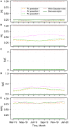
Preliminary assessment of the suitability of potential predictability measures for renewable generation time series (A), (B), (C), (D), and (E), respectively, show the values over time obtained by dispersion entropy (DE), permutation entropy (PE), sample entropy (SaE), spectral entropy (SpE), and weighted permutation entropy (WPE) for a sine wave signal (with a 1-day cycle), a white Gaussian noise (WGN), and three randomly selected PV generation time series from our dataset. These are calculated using 2-month rolling windows that move 1 day forward at a time. The hyperparameters are set to the commonly used values of each metric (i.e., the dimension of PE and WPE is 6, both the class and dimension of DE are 5, and the dimension of SE is 3).

Figure 2

Finding the best predictability measure and its hyperparameters for renewable generation time series Each line shows the average correlation between the predictability values obtained by a measure with a specific hyperparameter and 16 datasets of prediction errors, resulting from four prediction horizons (5 min, 10 min, 15 min, and 20 min ahead), two forecasting methods (ARIMA and naive), and two error metrics (NMAE and NRMSE).

Figure 3

High correlation between the WPE and the minutes-ahead prediction errors of solar PV generation The scatterplots show the relationship between the WPE of dimension 6 and the 10-min resampling interval, and the NRMSE and the NMAE of the PV generation data when ARIMA and naive forecasting methods are used to predict 5-, 10-, 15-, and 20-min-ahead generation.

Figure 4

Strong correlation between the WPE and the day-ahead prediction errors of solar PV generation The scatterplots show the relationship between the WPE of dimension 6 and the 10-min resampling interval, and the median NRMSE and the median NMAE of the day-ahead predictions of PV generation data using random forest and seasonal naive forecasting methods.

Figure 5

Australian electricity market regulation costs by type of power plant Each bar illustrates the share of power plants with a particular fuel type in the regulation FCAS costs of the Australian electricity market in each quarter of 2020. The shares of costs in each quarter are normalized by the terawatt-hours of generated energy during that period. The data for the regulation FCAS costs and the generation of each fuel type are collected from AEMO and OpenNEM, respectively.

Figure 6

Dependency of solar farms’ regulation market costs on the predictability of PV generation These plots show the relationship over time between the predictability (1 − WPE) of PV generation and the solar farms’ causer pays factors (CPFs) in New South Wales (NSW) over the year 2019. In (A), the PV generation data in NSW from our dataset is used to calculate the average predictability over time. However, in (B), the average predictability of PV generation is determined based on the predictability of global tilted irradiance (GTI) sun-tracking data in the exact locations of the six solar farms in NSW. The predictability of PV generation is calculated over 2-month rolling horizons with 1-month shifting forward. To make the CPF data comparable with the predictability values, we calculate the 2-month moving average of the CPF values of solar farms in the same way. The CPF data of solar farms in 2019 is gathered for every solar farm in NSW with a generation capacity above 10 MW, which are commissioned in or before January 2019, namely Griffith, Royalla, Mugga Lane, Manildra, Coleambally, and Moree solar farms. Also, the average CPF of solar farms and the predictability of monthly GTI data are calculated by the weighted average of the six farms based on their maximum generation capacity.

Figure 7

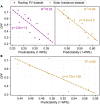
Strong inverse correlation between the regulation market costs and the generation predictability of solar farms In (A), the scatterplots illustrate the relationship between the average predictability and CPF of 2-month rolling horizons for the rooftop PV generation and the GTI dataset (the same data as in Figure 6). In (B), the scatterplot shows the relationship between the predictability of the solar farms’ GTI data and CPF for the six solar farms in NSW in the year 2019. The CPFs are normalized based on the capacity of each solar farm. In all scatterplots, the correlation between the two variables is statistically significant (p < 0.05); thus, the $R^2$ value is shown. Also, in each plot the linear regression equation describing the quantitative relationship between the CPF and the predictability is presented using the ordinary least squares method.

Figure 8

Annual solar irradiance and predictability values of (potential) solar farms in NSW In (A), the fill color of the circles quantifies the total annual GTI sun-tracking values for the potential solar farm locations in NSW. In (B), the fill colors of the circles quantify the predictability (1 − WPE) of the GTI data at the potential solar farm locations in NSW. The circles with orange borders indicate actual farm locations. Both the annual solar irradiance and predictability are calculated based on the 5-min GTI time series from August 2021 to August 2022. The GTI data were obtained from SolCast..

Figure 9

Impact of considering the predictability in choosing the best location for building a solar farm The bar plot shows the projected revenue changes of a 51.8 MW solar farm when installed in different locations, shown in Figure 8, with respect to location 1. In the first scenario, the revenue only depends on the annual solar irradiance. In the second scenario, the costs associated with the regulation market costs are also taken into account based on the changes in the predictability; thus, the CPF.

Figure 10

Impact of location on the predictability of solar PV generation The predictability values are shown for the 1-year PV generation of houses in different regions across Australia. Each region consists of postcodes within 25 km of each other. The circles on the maps are colored based on the average predictability (1 − WPE) of PV systems in that region. The resampling interval of the PV generation time series is 10 min, and the embedding dimension in the WPE calculation is set to 6.

Figure 11

Predictability and density of rooftop PV generation in SA A comparison between the PV generation predictability at SA’s local government areas (LGAs) with available data and the density of the dwellings with rooftop PV in the LGAs. The data for rooftop density is obtained from the Australian PV Institute. Also, the resampling interval of the PV generation time series is 10 min, and the embedding dimension of WPE is 6.

Figure 12

Different patterns of changes in PV generation predictability over time in different states of Australia The predictability values (1 − WPE) of a 2-month rolling horizon across a year for the PV systems’ generation profiles in the states of (A) SA, (B) VIC, and (C) NSW. In this analysis, the resampling interval of the PV generation time series is 10 min, and the embedding dimension of the WPE is 6.

References

1. World energy outlook 2022 . International Energy Agency; 2022. https://www.iea.org/reports/world-energy-outlook-2022 IEA.
1. End of coal in sight as UK secures ambitious commitments at COP26 summit . 2021. https://www.gov.uk/government/news/end-of-coal-in-sight-as-uk-secures-am...
1. Delarue, E., and Morris, J. Renewables intermittency: operational limits and implications for long-term energy system models. MIT Joint Program on the Science and Policy of Global Change (2015). URL: https://globalchange.mit.edu/sites/default/files/MITJPSPGC_Rpt277.pdf.
1. Managing Large-Scale Penetration of Intermittent Renewables . MIT Energy Initiative; 2012. https://energy.mit.edu/wp-content/uploads/2012/03/MITEI-RP-2011-001.pdf
1. South Australia’s Energy Solution . Government of South Australia; 2020. https://www.energymining.sa.gov.au/__data/assets/pdf_file/0009/364266/20...
LinkOut - more resources