Biobank-scale inference of ancestral recombination graphs enables genealogical analysis of complex traits

Abstract

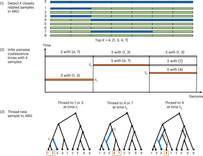
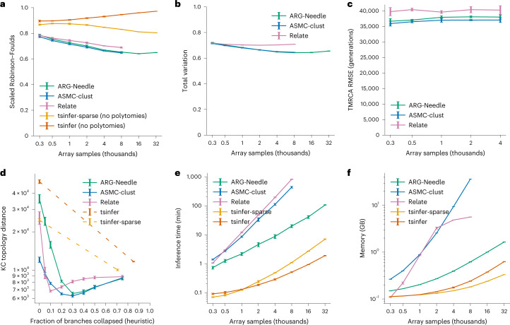
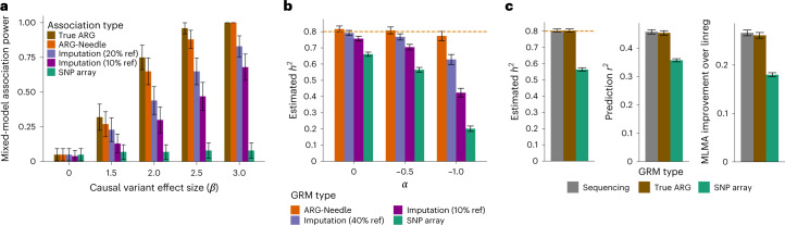
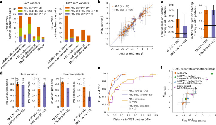
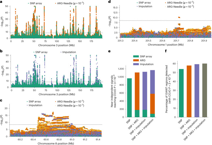
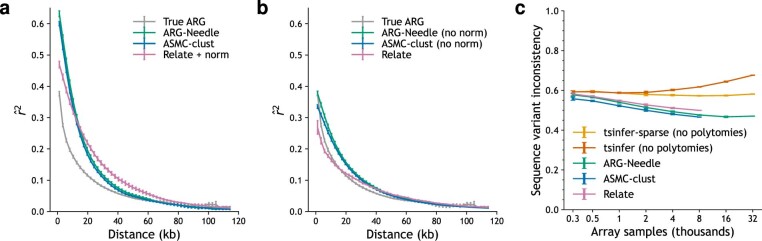
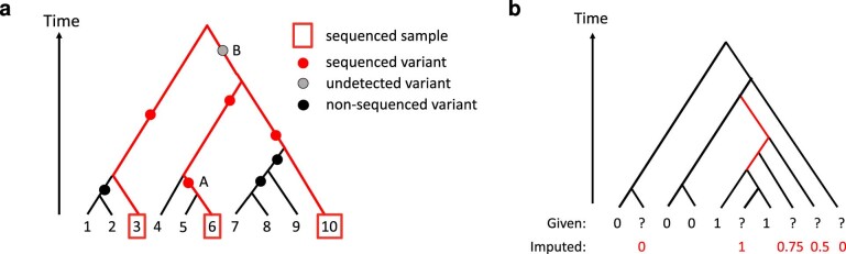
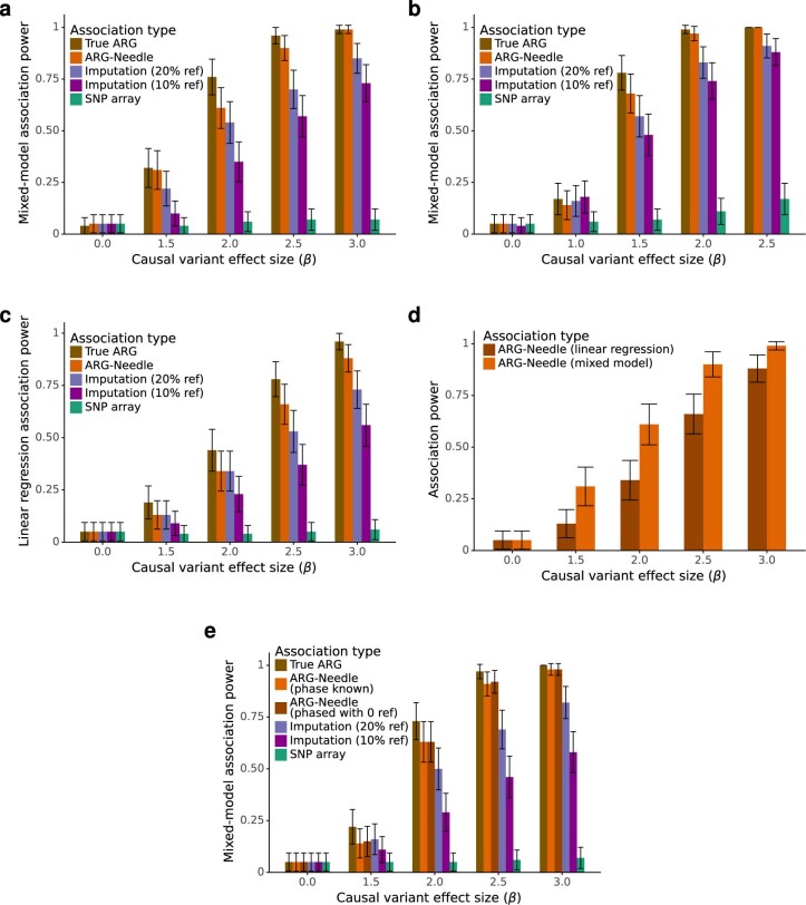
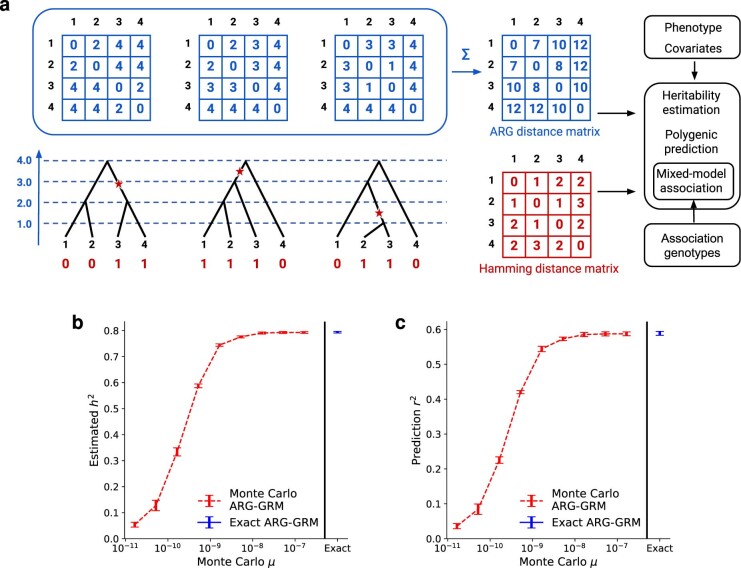
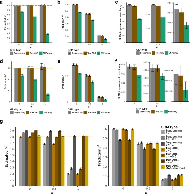
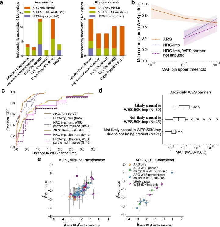
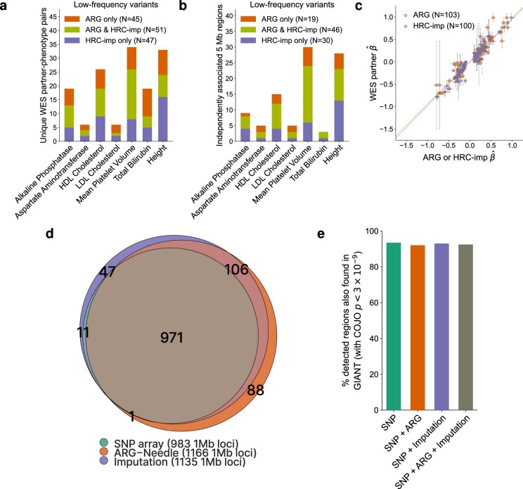
Genome-wide genealogies compactly represent the evolutionary history of a set of genomes and inferring them from genetic data has the potential to facilitate a wide range of analyses. We introduce a method, ARG-Needle, for accurately inferring biobank-scale genealogies from sequencing or genotyping array data, as well as strategies to utilize genealogies to perform association and other complex trait analyses. We use these methods to build genome-wide genealogies using genotyping data for 337,464 UK Biobank individuals and test for association across seven complex traits. Genealogy-based association detects more rare and ultra-rare signals (N = 134, frequency range 0.0007-0.1%) than genotype imputation using ~65,000 sequenced haplotypes (N = 64). In a subset of 138,039 exome sequencing samples, these associations strongly tag (average r = 0.72) underlying sequencing variants enriched (4.8×) for loss-of-function variation. These results demonstrate that inferred genome-wide genealogies may be leveraged in the analysis of complex traits, complementing approaches that require the availability of large, population-specific sequencing panels.

Fig. 1. Overview of the ARG-Needle algorithm.

ARG-Needle adds one haploid sample at a time to an existing ARG, each time performing three steps: (1) shortlisting a subset of most related samples already in the ARG through genotype hashing, (2) obtaining pairwise coalescence time estimates with these samples using ASMC and (3) using the ASMC output to ‘thread’ the new sample to the ARG. We depict an example of adding sample S to an ARG, focusing on one genomic region. Step 1 divides the genome into ‘words’ and checks for identical matches with sample S. Based on these matches (shown in blue), samples 1, 3, 4 and 7 are output as the K = 4 candidate most related samples already in the ARG. Step 2 computes pairwise coalescence time estimates between sample S and each of the samples 1, 3, 4 and 7. The minimum time for each position is highlighted. Step 3 uses these minimum times and samples to define a ‘threading instruction’ that is performed to add sample S to the ARG. Threading connects the new sample to the ancestral lineage of each chosen sample at the chosen time. Dotted lines indicate previous ARG edges that are inactive due to recombination. When all samples have been threaded, ARG-Needle performs a final postprocessing step called ARG normalization (Methods).

Fig. 2. Comparison of ARG inference algorithms in simulation.

a–f, We benchmark ARG inference performance for ARG-Needle, ASMC-clust, Relate, tsinfer and a variation of tsinfer for sparse data (‘tsinfer-sparse’) in realistic CEU demography array data simulations across a variety of metrics related to accuracy and computational resources (lower values indicate better performance for all metrics). a, The Robinson–Foulds distance (polytomies are randomly resolved). b, The ARG total variation distance (Methods). c, Pairwise TMRCA RMSE. d, The KC topology-only metric. e, Runtime. f, Peak memory. In c, we only run up to N = 4,000 haploid samples. In d, we fix N = 4,000 haploid samples and vary the fraction of branches per marginal tree that are collapsed to form polytomies, using a heuristic that preferentially collapses branches that are less confidently inferred (Methods). For tsinfer and tsinfer-sparse, we instead rely on the default amount of polytomies in the output, additionally showcasing when polytomies are randomly resolved (dashed lines indicate a linear trend that may not hold). All panels use five random seeds, with ASMC-clust and Relate capped at N = 8,000 haploid samples due to runtime or memory constraints. Data are presented as mean values ± 2 s.e.m. Relate’s default settings cap the memory for intermediate computations at 5 GB (see f). ARG-Needle and ASMC-clust include ARG normalization by default (Methods), while Relate does not. For additional simulations, see Extended Data Figs. 1–4 and Supplementary Figs. 1–6.

Fig. 3. ARG-based analysis of simulated complex traits.

a, Power to detect a rare causal variant (MAF = 0.025%) in simulations of a polygenic phenotype. We compare ARG-MLMA of ground-truth ARGs and ARG-Needle-inferred ARGs with MLMA of imputed and SNP array variants as we vary the effect size β (100 independent simulations of h² = 0.8, α = −0.25, N = 20,000 haploid samples and 22 chromosomes of 5 Mb each; Methods). b, Heritability estimation using ARG-GRMs from ARG-Needle inference on SNP array data, compared with using imputed or array SNPs (5 simulations of 25 Mb, N = 5,000 haploid samples, h² = 0.8 and varying α). c, ARG-GRMs computed using ground-truth ARGs perform equivalently to GRMs computed using sequencing data in heritability estimation, polygenic prediction and mixed-model association (N = 10,000 haploid samples, h² = 0.8 and α = −0.5). Heritability and prediction involve 5 simulations of 50 Mb, and association involves 50 simulations of 22 chromosomes of 2.5 Mb each, for a total of 55 Mb. For association, we show the relative improvement in mean −log₁₀(P) of MLMA compared with linear regression (Methods). ‘% ref’ indicates the size of the reference panel used for imputation as a percentage of the number of haploid samples (N = 20,000 in a, N = 5,000 in b). Data are presented as estimates ± 2 s.e.m., where the estimates are from meta-analysis in the case of heritability estimation, represent fractions in a and represent means otherwise. Additional results are shown in Extended Data Figs. 6–8 and Supplementary Fig. 8. linreg, linear regression.

Fig. 4. Association of ARG-derived and imputed rare and ultra-rare variants with seven quantitative traits in UK Biobank.

a, Counts of unique WES partners for ARG and HRC + UK10K-imputed (‘HRC-imp’) independent associations, partitioned by traits and frequency and showing overlap. Total bilirubin was not associated at these frequencies and height was not associated for ultra-rare variants. b, Scatter plot of $\widehat{\beta }$ (estimated effect) for independent variants (estimated within 337,464 samples) against $\widehat{\beta }$ for their WES partners (estimated within 138,039 samples), with linear model fit. c, Fraction of loss-of-function and other protein-altering variants for the unique WES partners of independent variants (125 WES partners for ARG and 62 for imputed variants). Horizontal black lines represent averages across exome sequencing variants. d, Average per-variant precision and recall of predicting WES carrier status, partitioned by frequency and showing individual value as jittered points (71 rare ARG, 53 rare imputed, 62 ultra-rare ARG and 12 ultra-rare imputed variants). e, Cumulative distribution function (CDF) for the distance between independent variants and their WES partners. f, Scatter plot of $\widehat{\beta }$ for ARG-derived independent variants associated with aspartate aminotransferase in the GOT1 gene (estimated within 337,464 samples) against $\widehat{\beta }$ for their WES partners (estimated within 138,039 samples). We color points based on whether the WES partner is likely causal in WES-50K-imp (imputation from WES-50K into ~459,000 samples), not likely causal but marginally significant in WES-50K-imp or not marginally significant in WES-50K-imp (‘ARG only’). We also plot the $\widehat{\beta }$ for the additional likely causal variants in WES-50K-imp against the $\widehat{\beta }$ in WES-138K. Bars represent fractions in c and means in d. Error bars represent 1.96 s.e.m. in b and f and represent bootstrap 95% CIs in c and d. Additional results are shown in Extended Data Fig. 9. HDL, high-density lipoprotein; LDL, low-density lipoprotein.

Fig. 5. Genealogy-wide association of higher frequency variants with height in UK Biobank.

a,b, Chromosome 3 Manhattan plots showing MLMA of ARG-Needle on SNP array data versus array SNPs (a) and HRC + UK10K-imputed variants versus array SNPs (b). c,d, Manhattan plots of two loci. c, ARG-MLMA detects haplotype structure that is found using imputation, with a different association peak. d, An association peak found by ARG-MLMA that was significant (P < 3 × 10⁻⁹) in a GIANT consortium meta-analysis of ~700,000 samples. e,f, Approximately independent associations (defined as having COJO P < 3 × 10⁻⁹; Methods) when considering array SNPs alone, array SNPs and ARG-Needle variants, array SNPs and imputed variants, and all three types of variants. e, Total number of independent variants found and attribution based on data type. f, Percentage of 1-Mb regions containing COJO associations in the GIANT meta-analysis that are detected using each method. For the Manhattan plots, the order of plotting is ARG-Needle with μ = 10⁻³ (used for follow-up), then ARG-Needle with μ = 10⁻⁵ (used for discovery), then imputation, then SNP array variants on top. Dotted lines correspond to P = 3 × 10⁻⁹ (Methods) and triangles indicate associations with P < 10⁻⁵⁰. See also Supplementary Figs. 9 and 10.

Extended Data Fig. 1. Additional comparison of ARG inference methods with array data and topology-only metrics.

We compare methods on runtime and topology-only metrics, as in Fig. 2 but with additional simulation conditions. All columns are for 5 Mb of CEU demography array data, and individual columns represent standard parameters (see Methods), a factor of 2 smaller recombination rate (ρ = 6 × 10⁻⁹), a factor of 2 larger recombination rate (ρ = 2.4 × 10⁻⁸), and a constant population size demography of 15,000 individuals. a. Robinson-Foulds distance as a function of the number of samples N, where values are scaled to lie between 0 and 1 (polytomies are randomly resolved). b. KC topology-only distance for N = 4,000 samples, showing performance as branches in marginal inferred trees are collapsed to form polytomies, using a heuristic to preferentially collapse branches that are least certain (see Methods). For tsinfer and tsinfer-sparse, we instead rely on the default amount of polytomies in the output, additionally showcasing when polytomies are randomly resolved (dashed lines indicate a linear trend may not hold). c. The same as b, except branches are randomly collapsed to form polytomies. d. KC topology-only distance as a function of N, with polytomies randomly resolved. e. Inference time as a function of N. All panels use 5 random seeds. Data are presented as means ± 2 s.e.m.

Extended Data Fig. 2. Additional comparison of ARG inference methods with array data and two branch length-aware metrics.

We compare methods as in Fig. 2b, c, but with additional simulation conditions. All columns are for 5 Mb of CEU demography array data, and individual columns represent standard parameters (see Methods), a factor of 2 smaller recombination rate (ρ = 6 × 10⁻⁹), a factor of 2 larger recombination rate (ρ = 2.4 × 10⁻⁸), and a constant population size demography of 15,000 individuals. We show results for the ARG total variation distance (a-b) and pairwise TMRCA RMSE (c-d), with (a,c) and without (b,d) ARG normalization, as these metrics are sensitive to branch length. All panels use 5 random seeds. Data are presented as means ± 2 s.e.m.

Extended Data Fig. 3. Comparison of ARG inference methods with sequencing data.

Simulations use 1 Mb of CEU sequencing data and otherwise standard parameters (see Methods). Individual panels correspond to rows of Extended Data Figs. 1a, 2a–d, and 1b–e, in that order, with the same metrics used, namely a. scaled Robinson-Foulds distance (polytomies are randomly resolved), b-c. ARG total variation distance with (b) and without (c) ARG normalization, d-e. pairwise TMRCA RMSE with (d) and without (e) ARG normalization, f-g. KC topology-only distance for N = 4,000 samples with heuristic (f) and random (g) collapsing of branches, h. KC topology-only distance with polytomies randomly resolved, and i. inference time. d,e use 25 random seeds, whereas all other panels use 5 random seeds. Data are presented as means ± 2 s.e.m.

Extended Data Fig. 4. Consistency of inferred ARGs with underlying linkage patterns and sequence-level variation.

a,b. Linkage disequilibrium (LD) decay up to 120 kilobases for ground truth ARGs as well as ARGs inferred by ARG-Needle, ASMC-clust, and Relate. LD was evaluated by placing mutations with a mutation rate of 5 × 10⁻⁸ per base pair per generation and filtering to variants with MAF > 5%. Lines show mean r² as a function of distance between variants, averaging across 10 independent simulations. Simulations were of 5 Mb of CEU demography array data with standard simulation parameters (see Methods). Methods including ARG normalization are shown in a, and methods without ARG normalization are shown in b, as branch lengths affect the probability for mutations to be sampled. c. We compute the fraction of underlying sequencing sites, of which the array variants are a subset, that cannot be mapped to branches of inferred ARGs (lower is better). Inference is on 5 Mb of CEU demography array data simulated with standard parameters (see Methods), averaging over 5 random seeds. no polytomies refers to randomly resolving polytomies of tsinfer and tsinfer-sparse (see Methods). Data are presented as means ± 2 s.e.m.

Extended Data Fig. 5. A genealogical view of genotype imputation and an algorithm for ARG-based imputation.

a. The marginal tree represents the relationships of 10 haploid samples and variant ages at a locus. 3 of the 10 samples are sequenced and used as a reference panel to impute sequenced variants into the remaining samples. An imputation algorithm may recognize sample 6 as the closest relative in the reference panel for samples 4 and 5, but if TMRCAs and variant times are not modeled, it may incorrectly impute variant ‘A’ into sample 4. Variant ‘B’ may represent a high frequency variant that is not present in the sequencing panel (for example, an undetected indel or structural variant). Non-sequenced variants cannot be imputed. All variants may be tested for association using branches of an accurately inferred genealogy. b. Schematic of an ARG-based imputation algorithm (see Supplementary Fig. 12 for exploratory results). Given a polymorphic sequenced site containing sequenced samples, unobserved genotypes for array samples, and a marginal tree relating all samples, we perform genotype imputation as follows. We first identify all branches in the tree for which a mutation on that branch best explains the observed sequencing data in terms of Hamming distance (red branches in the example). Each branch implies genotypes of 0 or 1 for the array samples, and we weight by branch length to produce a weighted predicted dosage for each array sample. In this example, the three branches have lengths in ratio 1:1:2, resulting in the predicted dosages shown in red.

Extended Data Fig. 6. Additional simulations of ARG-MLMA genealogy-wide association power.

a. Similar to Fig. 3a, except with a low-frequency causal variant (MAF = 0.05%) and a smaller simulation with N = 10,000 haploid samples and 22 chromosomes of 2.5 Mb each. b. Similar to a, except with the causal variant MAF chosen to be 0.1%. c. Similar to a, except using linear regression instead of the linear mixed model to test for association. d. We combine the association power results of ARG-Needle association from a and c, highlighting the improvement of ARG-MLMA compared to directly testing ARG clades using linear regression. e. As in a, but with N = 10,000 diploid instead of N = 10,000 haploid individuals. ARG-Needle is run with the true phase known and with reference-free phasing. % ref indicates the size of the reference panel used for imputation as a percentage of the number of haploid samples (N = 10,000 in a-c, 2 N = 20,000 in e). All panels use 100 independent simulations to measure power. Data are presented as fractions ± 2 s.e.m.

Extended Data Fig. 7. Overview of ARG-GRM definition and Monte Carlo estimator.

a. Schematic of ARG-GRMs. Given an ARG between samples, we can compute the TMRCA matrix at each site and sum this over the genome to obtain the α = 0 ARG distance matrix (top, in blue). This equals a scaled version of the expected Hamming distance matrix (bottom, in red), which is formed by counting the number of differences between the genotypes of samples. By applying a series of simple matrix transformations to the ARG distance matrix (see Supplementary Note 3), we obtain the ARG-GRM, which can subsequently be used in complex trait analysis just like genotype-based GRMs. b,c. We compare the use of an exact α = 0 ARG-GRM to Monte Carlo α = 0 ARG-GRMs for heritability estimation (b) and polygenic prediction (c). As we increase the mutation rate for the Monte Carlo ARG-GRMs (rightmost value of μ = 1.65 × 10⁻⁷), we approach results from using the exact ARG-GRM. Shown are 5 independent simulations of N = 2,000 haploid samples, h² = 0.8, α = 0, 10 Mb. Data are presented as estimates ± 2 s.e.m., where the estimates are from meta-analysis in the case of heritability estimation and represent means otherwise.

Extended Data Fig. 8. Additional simulations for ground-truth ARG-GRMs.

a-f. As in Fig. 3c, with N = 10,000 haploid samples, except we vary h² ∈ {0.8, 0.3} and α ∈ {0, −0.5, −1}. a, d. Heritability estimation for a 50 Mb region for h² = 0.8 (a) and h² = 0.3 (d). b, e. Polygenic prediction for a 50 Mb region for h² = 0.8 (b) and h² = 0.3 (e). c, f. Mixed-model association for 22 chromosomes of 2.5 Mb each for h² = 0.8 (c) and h² = 0.3 (f). g. Panels a-f assumed it is possible to infer α and used the true α when building genotype-based or ARG-GRMs. If this value of α is misspecified, heritability estimation is biased and prediction r² is hampered. This is true both for ARG-GRMs and sequencing GRMs. However, using MAF-stratified ARG-GRMs provides a robust way to estimate the true heritability when α is unknown, and achieves prediction r² comparable to using the true α (N = 10,000 haploid samples, 50 Mb, h² = 0.8). For all panels, heritability and prediction experiments involve 5 simulations per bar, and most association experiments involve 50 simulations per bar, except for the h² = 0.3, α = −1 condition in f, which involved 500 simulations. Data are presented as estimates ± 2 s.e.m., where the estimates are from meta-analysis in the case of heritability estimation and represent means otherwise. Prediction r² for individual simulations is shown in b and e.

Extended Data Fig. 9. Further results for rare and ultra-rare variant associations.

a. Counts of implicated 5 Mb regions containing ARG and HRC + UK10K imputation (‘HRC-imp’) independent associations, partitioned by traits and frequency and showing overlap. Total bilirubin was not associated at these frequencies. b. Average Pearson correlation between independent variants and their WES partners as a function of frequency, for ARG-derived variants, HRC + UK10K imputed variants, and HRC + UK10K imputed variants for which the WES partner was not the imputed variant. Dots represent the upper end of a frequency range. Central lines represent means and shaded areas represent 95% bootstrap confidence intervals. c. Cumulative distribution function for the distance between independent variants and their WES partners, partitioned by frequency. As in Fig. 4b, but also showing HRC + UK10K imputed variants for which the WES partner was not the imputed variant. d. Box plots of MAF for WES partners found by ARG-derived but not HRC + UK10K imputed independent variants (center line, median; box limits, upper and lower quartiles, whiskers, 1.5× interquartile range; points, outliers), stratifying by status in WES-50K-imp (imputation from WES-50K). e. Scatter plot of $\widehat{\beta }$ (estimated effect) for ARG-derived independent variants (estimated within 337,464 samples) against $\widehat{\beta }$ for their WES partners (estimated within 138,039 samples), as in Fig. 4f but for associations with alkaline phosphatase in the ALPL gene and with LDL cholesterol in the APOB gene. We color points based on whether the WES partner is likely causal in WES-50K-imp, not likely causal but marginally significant in WES-50K-imp, or not marginally significant in WES-50K-imp (‘ARG only’ in figure). We also plot the $\widehat{\beta }$ for the additional likely causal variants in WES-50K-imp against the $\widehat{\beta }$ in WES-138K. Error bars represent 1.96 s.e.m.

Extended Data Fig. 10. Additional results for low (0.1% ≤ MAF < 1%) and high frequency (MAF ≥ 1%) variant associations.

a-c. Association of ARG-derived and imputed low-frequency variants with 7 quantitative traits. a. Counts of unique WES partners for ARG and HRC + UK10K imputed (‘HRC-imp’) independent associations, partitioned by traits and showing overlap. b. Counts of implicated 5 Mb regions containing ARG and HRC + UK10K imputation independent associations, partitioned by traits and showing overlap. c. Scatter plot of estimated effect ($\widehat{\beta }$) for independent variants (estimated within 337,464 samples) against $\widehat{\beta }$ for their WES partners (estimated within 138,039 samples), with linear model fit. Error bars represent 1.96 s.e.m. d, e. Association of higher frequency variants with height. d. Venn diagram of number of 1 Mb regions containing a significant hit at P < 3 × 10⁻⁹ for ARG-Needle (MAF ≥ 1%, μ = 10⁻⁵), HRC + UK10K imputed (MAF ≥ 0.1%, info score > 0.3) and SNP array association. ARG-Needle association detected 971 out of 982 (98.9%) 1 Mb regions found by both imputation and array, 108 out of 153 (71%) 1 Mb regions found by imputation but not array and an additional 92 (8% increase upon 1140) 1 Mb regions to those already found by imputation and array. e. Percent of 1 Mb regions containing independent associations (defined as having COJO P < 3 × 10⁻⁹, see Methods) in association scans of 337,464 UK Biobank individuals that were also present in a GIANT consortium meta-analysis of ∼700,000 samples.

References

1. Bamshad M, Wooding SP. Signatures of natural selection in the human genome. Nat. Rev. Genet. 2003;4:99–110. - PubMed
1. Beichman AC, Huerta-Sanchez E, Lohmueller KE. Using genomic data to infer historic population dynamics of nonmodel organisms. Annu. Rev. Ecol. Evol. Syst. 2018;49:433–456.
1. Browning SR, Browning BL. Haplotype phasing: existing methods and new developments. Nat. Rev. Genet. 2011;12:703–714. - PMC - PubMed
1. Marchini J, Howie B. Genotype imputation for genome-wide association studies. Nat. Rev. Genet. 2010;11:499–511. - PubMed
1. McVean GA, Cardin NJ. Approximating the coalescent with recombination. Philos. Trans. R. Soc. Lond. B Biol. Sci. 2005;360:1387–1393. - PMC - PubMed
Publication types