Multidimensional cerebellar computations for flexible kinematic control of movements

Abstract

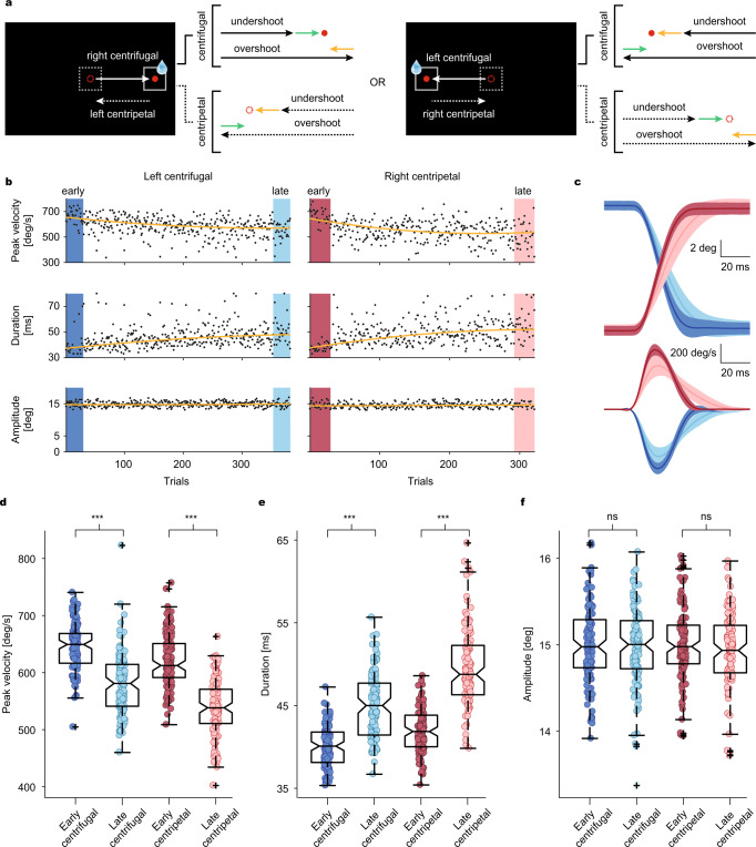
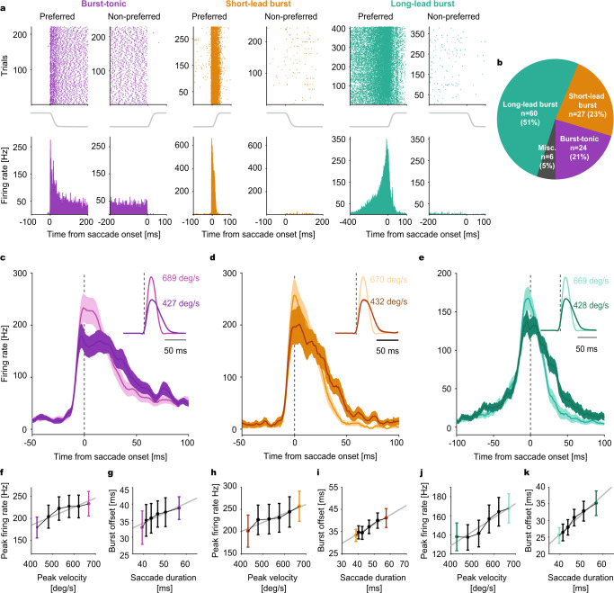
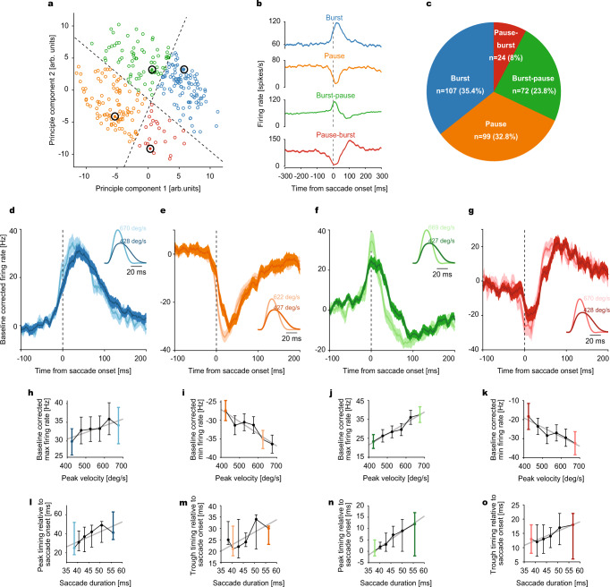
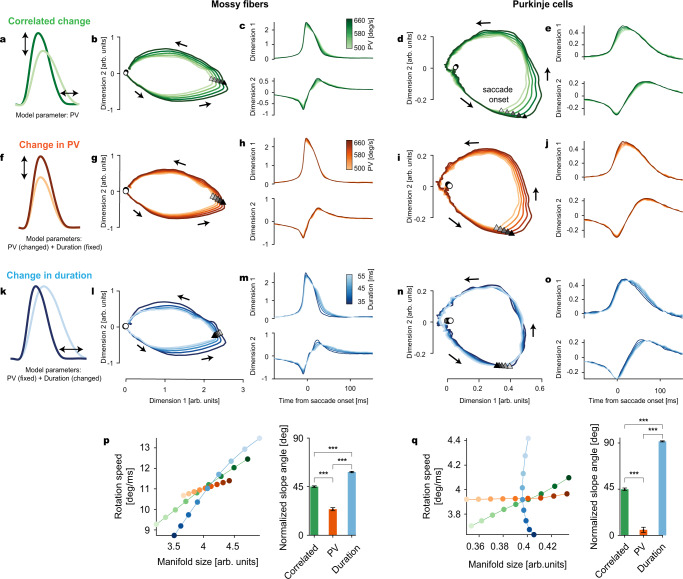
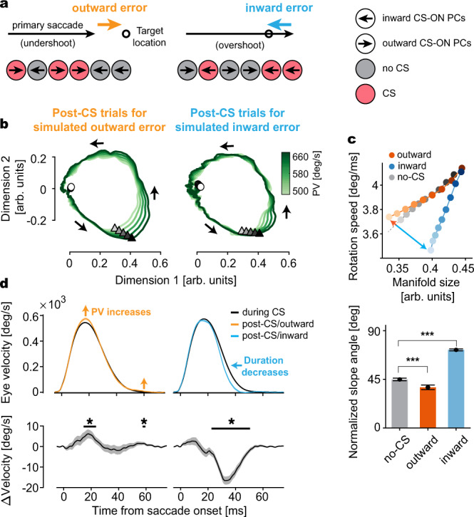
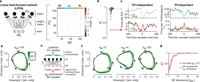
Both the environment and our body keep changing dynamically. Hence, ensuring movement precision requires adaptation to multiple demands occurring simultaneously. Here we show that the cerebellum performs the necessary multi-dimensional computations for the flexible control of different movement parameters depending on the prevailing context. This conclusion is based on the identification of a manifold-like activity in both mossy fibers (MFs, network input) and Purkinje cells (PCs, output), recorded from monkeys performing a saccade task. Unlike MFs, the PC manifolds developed selective representations of individual movement parameters. Error feedback-driven climbing fiber input modulated the PC manifolds to predict specific, error type-dependent changes in subsequent actions. Furthermore, a feed-forward network model that simulated MF-to-PC transformations revealed that amplification and restructuring of the lesser variability in the MF activity is a pivotal circuit mechanism. Therefore, the flexible control of movements by the cerebellum crucially depends on its capacity for multi-dimensional computations.

Fig. 1. Repetitive saccade task induces a gradual decline in saccade velocity.

a Behavioral task. Saccades were made repetitively, either in left or right directions. All center-out (centrifugal (CF), solid arrows) saccades were rewarded. Centripetal (CP) saccades (dashed arrows) were not rewarded. Both CF and CP saccades could lead to errors in leftward (orange arrows) or rightward (green arrows) directions. b Gradual decay of peak velocity (upper panels) in CF (left) and CP (right) saccades (CF: p = 1.12 × 10⁻⁵, Z = 4.4; CP: p = 1.02 × 10⁻⁵, Z = 4.4) is paralleled by an increase in duration (middle panels, CF: p = 1.82 × 10⁻⁴, Z = −3.7; CP: p = 1.9 × 10⁻⁶, Z = −4.8) to stabilize amplitudes (lower panels, CF: p = 0.89, Z = −0.1; CP: p = 0.95, Z = 0.1) within a single session. Comparison based on n = 30 early and late trials, respectively. Each dot represents data from a single trial. Trends in the data are highlighted by fitting second-order polynomial fits (dark yellow lines) to the data. All comparisons based on two-sided Wilcoxon signed-rank tests. c Comparison of horizontal eye position and velocity profiles of early (i.e., first 30 trials, CF: dark blue; CP: dark red) and late (i.e., last 30 trials, CF: light blue; CP: light red) trials chosen from the experimental session in b. Data are mean ± SD. d–f Population analysis of 117 behavioral sessions. Box plots showing overall reduction of peak velocity (CF: p = 6.51 × 10⁻¹⁸, Z = 8.6; CP: p = 8.81 × 10⁻²¹, Z = 9.3) in late trials (lighter colors) as compared to early (darker colors) ones which is compensated by the upregulation of saccade duration (CF: p = 1.31 × 10⁻²⁰, Z = −9.3; CP: p = 8.81 × 10⁻²¹, Z = −9.3) during the late trials to maintain amplitude around 15 deg (CF: p = 0.57, Z = 0.6; CP: p = 0.01, Z = 2.5). Each data point corresponds to the mean value of the early (first 30, dark-colored circles) and late (last 30, light-colored circles) CF (blue circles) and CP saccades (red circles) of an individual session (n = 117 sessions). All comparisons based on two-sided Wilcoxon signed-rank tests. Significant differences are highlighted by asterisks. On each boxplot, center is median value, lower and upper edges of the box are 25th and 75th percentiles, respectively, whiskers extend to extreme values and outliers are marked as “+”.

Fig. 2. Encoding of saccade kinematics by mossy fibers (MFs).

a Raster plots (up) and average firing histogram (bottom) of a representative burst-tonic (purple), short-lead burst (yellow) and long-lead burst (turquoise) MF unit. Solid gray lines between upper and lower panels are the mean horizontal eye position traces. Data are aligned to saccade onset. b Proportion of MF units in each category. c–e Population response of burst-tonic (purple), short-lead burst (yellow) and long-lead burst (turquoise) MFs to high and low velocity saccades (see insets for average velocity profiles), represented by lighter and darker shades, respectively. Solid lines represent the mean and the shaded regions are ±SEM. f, h, j Average peak firing rate as a linear function of saccade peak velocity (bin size = 50 deg/s) for each MF category. Linear regression parameters: Burst-tonic (f): p = 0.016, R² = 0.83; Short-lead burst (h): p = 0.005, R² = 0.9; Long-lead burst (j): p = 0.006, R² = 0.9. g, i, k Average burst offset relative to saccade onset as a function of saccade duration (calculated from velocity bins) for each MF category. Linear regression parameters: Burst-tonic (g): p = 0.008, R² = 0.88; Short-lead burst (i): p = 0.0005, R² = 0.96; Long-lead burst (k): p = 0.0005, R² = 0.97. Solid gray lines represent the linear regression fits. Light and dark-colored bins correspond to the high and low peak velocity bins, respectively, for which population responses in c, d and e are plotted for comparison. Data are mean ± SEM obtained from n = 24 burst-tonic, n = 60 long-lead burst and n = 27 short-lead burst units, respectively.

Fig. 3. Classification of simple spike (SS) responses of Purkinje cells (PCs) into different categories and their encoding of saccade kinematics.

a Scatter plot of the first two principal components of SS responses. Classification of PCs into four response categories: burst (blue), pause (orange), burst-pause (green) and pause-burst (red), separated by decision boundaries (dotted black lines). Each data point corresponds to a PC’s SS response in one of the two directions. b Saccade onset-aligned average SS responses of exemplary units taken from each category (large black circles in a). c The proportion of units in each category. d–g SS population response (baseline corrected, mean ± SEM) of all four categories to high and low velocity saccades (see insets for average velocity profiles), represented by lighter and darker shades, respectively. Data are aligned to saccade onset. h–k Baseline corrected, average maximum (h, j) and minimum (i, k) firing rates as a function of saccade peak velocity (bin size = 50 deg/s) for each category. Linear regression parameters: Burst (h): n = 107 units, p = 0.041, R² = 0.69; Pause (i): n = 99 units, p = 0.0068, R² = 0.87; Burst-pause (j): n = 72 units, p = 0.00081 R² = 0.95; Pause-burst (k): n = 24 units, p = 0.0059, R² = 0.88. l–o Average peak (for burst (n = 107) and burst-pause (n = 72) units; l, n) and trough (for pause (n = 99) and pause-burst (n = 24) units; m, o) timing relative to saccade onset as a function of saccade duration (calculated from velocity bins) for each PC category. Linear regression parameters: Burst (l): p = 0.065, R² = 0.61; Pause (m): p = 0.087, R² = 0.56; Burst-pause (n): p = 0.00015, R² = 0.98; Pause-burst (o): p = 0.0059, R² = 0.88. Solid gray lines represent the linear regression fits. Light and dark-colored bins correspond to the high and low peak velocity bins, respectively, for which population responses in d–g are plotted. Data are mean ± SEM.

Fig. 4. Manifolds identified in MF and PC-SS activity perform multi-dimensional encoding of eye movements.

a Correlated changes in peak velocity (PV) and duration when PV is used as the only control parameter. b 2D plot of the first two dimensions in the MF manifold. Triangles and circles mark the saccade onsets and 250 ms before saccade onsets, respectively. Arrows show the direction of rotation. c The first two dimensions in b, plotted in time. d, e Same as b, c for PCs. f Isolated changes in saccade PV with the duration kept constant. g, h Isolated PV-dependent changes in the MF manifold computed from the rate models parametrized by PV but with fixed duration. i, j Same as g, h for PCs. k Isolated changes in saccade duration with constant PV. l–o Same as g, h and i, j but for duration change. p Left: MF manifold size versus rotation speed along the MF manifold varying with the correlated (green; a) and independent (orange and blue; f, k) change of PV and duration. Colors are as the color bars in c, h, m. Right: slope angle of the lines in left. In computing the angles, the x- and y-coordinates (manifold size and rotation speed) are normalized by the standard deviation of the correlated change case. T-val (Correlated, PV) = 17.97; ***: p = 1.27 × 10⁻³⁵, T-val (PV, Duration) = −30.37; ***: p = 2.44 × 10⁻⁵⁷, T-val (Correlated vs Duration) = −19.18; ***: p = 4.46 × 10⁻³⁸. q Same as p for PCs. T-val (Correlated, PV) = 19.75; p = 5.26 × 10⁻⁴⁴, T-val (PV, Duration) = −47.18; p = 1.36 × 10⁻⁹², T-val (Correlated vs Duration) = −48.13; ***: p = 8.24 × 10⁻⁹⁴. p Values are from one-sided Student’s t tests. Data are jackknife mean ± SEM from n = 117 MFs and n = 151 PCs.

Fig. 5. Complex spike (CS)-driven plasticity of PC manifolds is error-state dependent and predicts eye movement change.

a Two different types of eye movement errors and CS firing in PCs encoding the errors. Left: An undershooting eye movement causes an outward error (orange) and CS firing in a population of PCs with the same CS-ON direction (red) but not in the other, CS-OFF PCs (gray). Right: Same as Left for an overshooting saccade causing an inward error (blue). b Left: PC manifolds reflecting the combined influence of simulated outward error-encoding CS firing pattern on a particular trial, obtained by combining CS trials of CS-ON PCs (red circles) and no-CS trials of CS-OFF PCs (gray circles), on subsequent trials. Note that, in simulated error trials we assume that CS-ON PCs reported an error by firing a CS during 50–140 ms after saccade offset, whereas CS-OFF PCs reported the same error by not firing a CS, irrespective of the actual presence of an error. Right: same as Left, but for the inward error. c Top: manifold size versus rotation speed after the outward (orange) and inward (blue) error-encoding CS trials, and after no-CS trials (gray). Color bar gradient represents PV from 500 deg/s (brightest) to 660 deg/s (darkest). Bottom: comparison of normalized slope angles for each condition. Data are jackknife mean ± SEM from n = 151 PCs. T-val (No-CS, Outward) = 4.11; ***: p = 3.18 × 10⁻⁵, T-val (Outward, Inward) = −20.76; ***: p = 2.20 × 10⁻⁴⁶, T-val (No-CS, Inward) = −25.33; ***: p = 1.54 × 10⁻⁵⁶. p Values are from one-sided Student’s t tests. d Top: average saccade velocity profiles in the CS (black) and post-CS trials (colored) for the simulated outward (left) and inward (right) errors. For highlighting the differences in velocity profiles, colored lines represent the cumulative effect of five CSs. Bottom: average eye velocity change from the CS to post-CS trials. Data are mean ± SEM. *p < 0.05 (two-sided Student’s t test).

Fig. 6. Linear feed-forward network (LFFN) model from MFs to PCs.

a Left: schematic diagram showing LFFN for MF-to-PC firing rate transformation. Right: weight matrix computed from the data. Horizontal color bars on the top correspond to the three MF categories (BT burst-tonic, LL long-lead burst, SL short-lead burst). b Goodness of fit (R²) for individual PCs. The horizontal bar represents the median and the vertical bar extends from the first to third quantile, respectively. Colored circles correspond to examples shown in c. c Firing rates of example PCs (black, top and bottom) and LFFN predictions (color). The baselines are subtracted in the PV-independent component (left). d LFFN prediction of PC manifolds in Fig. 4d using all dimensions in MF firing. e Schematic diagram of the LFFN model showing steps involved (from bottom to top) in the prediction of PC manifolds from d_MF-dimensional MF manifolds. f Examples of the predicted PC manifold from e when MF manifold dimension is d_MF = 2 (left), 4 (middle), and 20 (right). g Goodness of fit for the predicted PC manifold to the data versus the input MF manifold dimensions d_MF. Dots represent examples in f. Data are mean ± SEM.

References

1. McLaughlin SC. Parametric adjustment in saccadic eye movements. Percept. Psychophys. 1967;2:359–362. doi: 10.3758/BF03210071. - DOI
1. Golla H, et al. Reduced saccadic resilience and impaired saccadic adaptation due to cerebellar disease. Eur. J. Neurosci. 2008;27:132–144. doi: 10.1111/j.1460-9568.2007.05996.x. - DOI - PubMed
1. Markanday A, Messner J, Thier P. A loss of a velocity‐duration trade‐off impairs movement precision in patients with cerebellar degeneration. Eur. J. Neurosci. 2018;48:1976–1989. doi: 10.1111/ejn.14062. - DOI - PMC - PubMed
1. Prsa M, Dicke PW, Thier P. The absence of eye muscle fatigue indicates that the nervous system compensates for non-motor disturbances of oculomotor function. J. Neurosci. 2010;30:15834–15842. doi: 10.1523/JNEUROSCI.3901-10.2010. - DOI - PMC - PubMed
1. Barash S, et al. Saccadic dysmetria and adaptation after lesions of the cerebellar cortex. J. Neurosci. 1999;19:10931–10939. doi: 10.1523/JNEUROSCI.19-24-10931.1999. - DOI - PMC - PubMed
Publication types