Predicting cellular responses to complex perturbations in high-throughput screens

Abstract

Recent advances in multiplexed single-cell transcriptomics experiments facilitate the high-throughput study of drug and genetic perturbations. However, an exhaustive exploration of the combinatorial perturbation space is experimentally unfeasible. Therefore, computational methods are needed to predict, interpret, and prioritize perturbations. Here, we present the compositional perturbation autoencoder (CPA), which combines the interpretability of linear models with the flexibility of deep-learning approaches for single-cell response modeling. CPA learns to in silico predict transcriptional perturbation response at the single-cell level for unseen dosages, cell types, time points, and species. Using newly generated single-cell drug combination data, we validate that CPA can predict unseen drug combinations while outperforming baseline models. Additionally, the architecture's modularity enables incorporating the chemical representation of the drugs, allowing the prediction of cellular response to completely unseen drugs. Furthermore, CPA is also applicable to genetic combinatorial screens. We demonstrate this by imputing in silico 5,329 missing combinations (97.6% of all possibilities) in a single-cell Perturb-seq experiment with diverse genetic interactions. We envision CPA will facilitate efficient experimental design and hypothesis generation by enabling in silico response prediction at the single-cell level and thus accelerate therapeutic applications using single-cell technologies.

Keywords: generative modeling; high-throughput screening; machine learning; perturbation prediction; single-cell transcriptomics.

Figure 1. Interpretable single‐cell perturbation modeling using a compositional perturbation autoencoder (CPA)

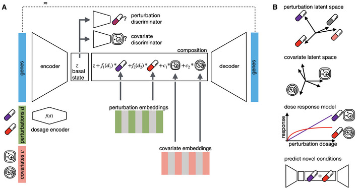
1. Given a matrix of gene expression per cell together with annotated potentially quantitative perturbations d and other covariates such as cell line, patient, or species, CPA learns the combined perturbation response for a single‐cell. It encodes gene expression using a neural network into a lower dimensional latent space that is eventually decoded back to an approximate gene expression matrix, as close as possible to the original one. To make the latent space interpretable in terms of perturbation and covariates, the encoded gene expression vector is first mapped to a “basal state” by feeding the signal to discriminators to remove any signal from perturbations and covariates. The basal state is then composed with perturbations and covariates, with potentially reweighted dosages, to reconstruct the gene expression. All encoder, decoder, and discriminator weights as well as the perturbation and covariate dictionaries are learned during training.

2. Features of CPA are interpreted via plotting of the two learned dictionaries, interpolating covariate‐specific dose–response curves and predicting novel unseen drug combinations.

Figure 2. Learning drug and cell line latent representations from massive single‐cell screens of 188 drugs across cancer cell lines

1. UMAP representation of sci‐Plex samples (n = 290,889) of A549, K562, and MCF7 cell‐lines colored by pathway targeted by the compounds to which cells were exposed.

2. Distribution of top 5 differentially expressed genes in A549 cells after treatment with Momelotinib, a JAK inhibitor, at the highest dose for real, control and CPA predicted cells.

3. Mean gene expression of 5,000 genes and top 50 DEGs between CPA predicted and real cells together with the top five DEGs highlighted in red for four compounds for which the model did not see any examples of the highest dose.

4. Box plots of $R^2$ scores for predicted and real cells for 36 compounds and 108 unique held out conditions across different cell lines. Baseline indicates comparison of each condition with a mean derived from randomly sampled cells.

5. $R^2$ scores box plot for all and top 50 DEGs. Each column represents a scenario where cells exposed with specific dose for all compounds on a cell line or combinations of cell lines were held out from training and later predicted.

6. Latent representation as learned by CPA of 82 cell lines from the L1000 dataset, with some cancer cell lines colored by tissue of origin.

7. Two‐dimensional representation of latent drug embeddings as learned by the CPA. Compounds associated with epigenetic regulation, tyrosine kinase signaling, and protein folding/degradation pathways are colored by their respectively known pathways. The smaller upper right panel shows latent covariate embedding for three cell lines in the data, indicating no specific similarity preference.

8. Latent drug embedding of CPA model trained on the bulk‐RNA cell line profiles of the top 1,000 most tested compounds from the L1000 dataset. Compounds overlapping with the sci‐Plex experiment in (A) are colored according to the same pathway labels as in (G).

Data information: Box plots in (E and F) indicate the median (center lines) and interquartile range (hinges), and whiskers represent minimum and maximum values.

Figure 3. Validation of predictions in new large‐scale drug combination dataset

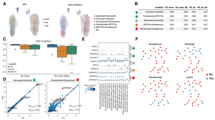
1. UMAP representation of the combosciplex dataset comprised of n = 63,378 cells and 32 perturbation and perturbation combinations in A549 cells. The left UMAP highlights the split used for the following results. The right UMAP shows the five out‐of‐distribution conditions selected and their expression pattern amongst the clusters.

2. The five out‐of‐distribution conditions shown in (A) and model performance per condition. The circles to the left of the condition names indicate a qualitative difficulty assessment of the prediction. Conditions with the green label are dominated by one of the two compounds in the condition and should be relatively easy for the model to predict, while combinations containing Alvespimycin are more transcriptionally dissimilar from conditions seen in training.

3. Benchmark of CPA vs. a linear model vs. the aforementioned random baseline, as measured by R2 on both highly variable genes and the top 50 differentially expressed genes. Box plots indicate the median (center lines) and interquartile range (hinges), and whiskers represents minimum and maximum values.

4. Predicted vs. true, post‐treatment expression values, with the top 5 DEGs colored in red.

5. Violin plots of the top two DEGs per out‐of‐distribution condition and the pre‐stimulation, post‐stimulation, and CPA predicted expression values.

6. UMAP representation of the combination latent vectors learned by CPA. Four individual conditions and the combinations they appear in are highlighted.

Figure 4. CPA extensibility enables predicting the response to unseen drugs

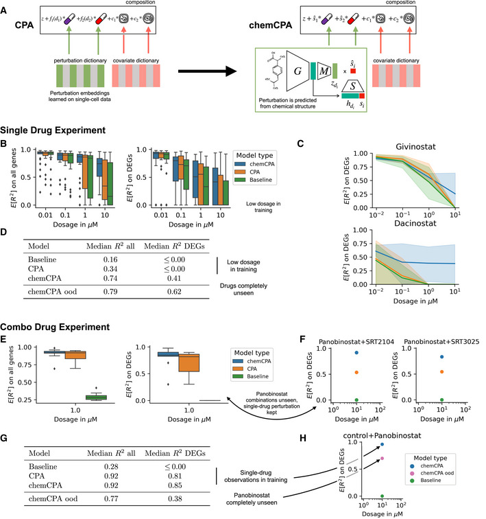
1. Proposed architecture change for CPA to include chemical prior knowledge. The molecule encoder $G$ maps the chemical information of a compound to a latent drug embedding $h_{d_i}$. This module can be based on a pre‐trained graph encoder or molecular fingerprints like here. During training only the perturbation module $M$ and the amortized dosage scaler $S$ are optimized.

2. Comparison between CPA and chemCPA, including a baseline that ignores all drug‐induced perturbation effects. Scores are computed on the sci‐Plex3 (n = 290,889) data on a test set that consists of nine compounds. Both the whole genes set (left) and the DEGs (right) are shown.

3. Performance comparison between the models from (B) for two histone deactylation drugs, Givinostat and Dacinostat, across all doses and cell‐lines (shades).

4. Median scores for the models from (B) for the highest dose value of 10 μM, including the result of chemCPA for the setting in which the nine test compounds are completely unseen and excluded from the training and validation.

5. Comparison between CPA and chemCPA on the new combosciplex (n = 63,378) including the same type of baseline as in (B). The test set consists of all nine drug combinations that include Panobinostat.

6. Detailed performance comparison between the models from (E) for the two conditions with the highest R2 difference on the DEGs.

7. Median scores for the models from (E), including the result of chemCPA where also the single‐drug Panobinostat observations were held‐out. The median score on the DEGs reduces from 0.85 to 0.38.

8. Showing how well chemCPA is able to predict the single‐drug effect of Panobinostat when it is held out. This is compared to the achieved score when Panobinostat is included in the training set (E).

Data information: Box plots indicate the median (center lines) and interquartile range (hinges), and whiskers represent minimum and maximum values.

Figure 5. Predicting combinatorial genetic perturbations

1. UMAP inferred latent space using CPA for 281 single and double‐gene perturbations obtained from Perturb‐seq (n = 108,497). Each dot represents a genetic perturbation. Coloring indicates known gene programs associated with perturbed genes from the original publications.

2. Measured and CPA‐predicted gene expression for cells linked to a synergistic gene pair (CBL + CNN1). Gene names taken from the original publication.

3. As (b) for an epistatic (DUSP9 + ETS) gene pair. Top 10 DEGs of DUSP9 + ETS co‐perturbed cells versus control cells are shown.

4. R2 values of mean gene‐expression of measured and predicted cells for all genes (black) or top 100 DEGs for the prediction of all 131 combinations for CPA, linear model, and the baseline (13 trained models, with ≈10 tested combinations each time).

5. R2 values of predicted and real mean gene‐expression versus number of cells in the real data.

6. R2 values for predicted and real cells versus number of combinations seen during training.

7. UMAP of mean gene expression in each measured (n = 284, red dots) and CPA‐predicted (n = 5,329, gray dots) perturbation combinations.

8. As (g), showing measurement uncertainty (cosine similarity).

9. As (g), showing dominant genes in Leiden clusters (25 or more observations). KLF1 cluster is highlighted with red dotted circle.

10. UMAP of mean expression of cells with KLF1 as a common co‐perturbed gene.

11. Hierarchical clustering of linear regression associated metrics between KLF1 with co‐perturbed genes, in measured and predicted cells. Each row indicates summary parameters obtained when fitting a linear regression for double predictions using single perturbations as predicting variables, and relationships between coefficients c₁ and c₂. For definitions see Materials and Methods.

12. Scaled gene expression changes (versus control) of RF‐selected genes (x‐axis) in measured (purple) and predicted (yellow) perturbations (y‐axis). Headers indicate gene‐wise regression coefficients, and interaction mode suggested by (Norman et al, 2019).

Data information: Box plots indicate the median (center lines) and interquartile range (hinges), and whiskers represent minimum and maximum values.

References

-
- Al‐Lazikani B, Banerji U, Workman P (2012) Combinatorial drug therapy for cancer in the post‐genomic era. Nat Biotechnol 30: 679–692 - PubMed
- van den Brink SC, Alemany A, van Batenburg V, Moris N, Blotenburg M, Vivié J, Baillie‐Johnson P, Nichols J, Sonnen KF, Arias AM et al (2020) Single‐cell and spatial transcriptomics reveal somitogenesis in gastruloids. Nature 582: 405–409 - PubMed
Publication types
MeSH terms
LinkOut - more resources
Full Text Sources
Other Literature Sources
Molecular Biology Databases