Profiling the human intestinal environment under physiological conditions

Abstract

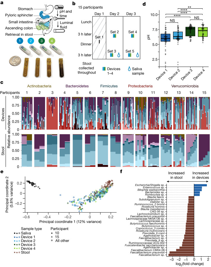
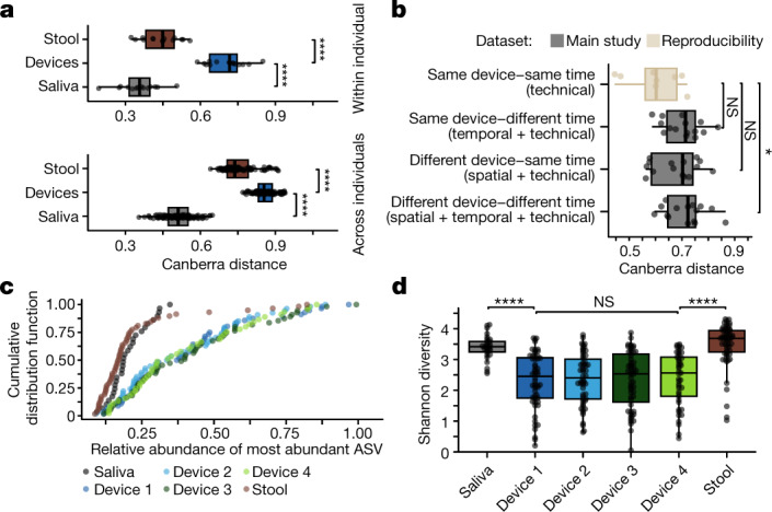
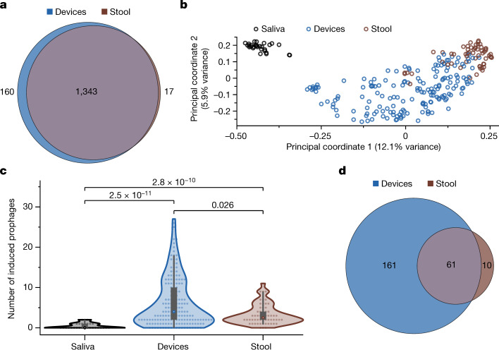
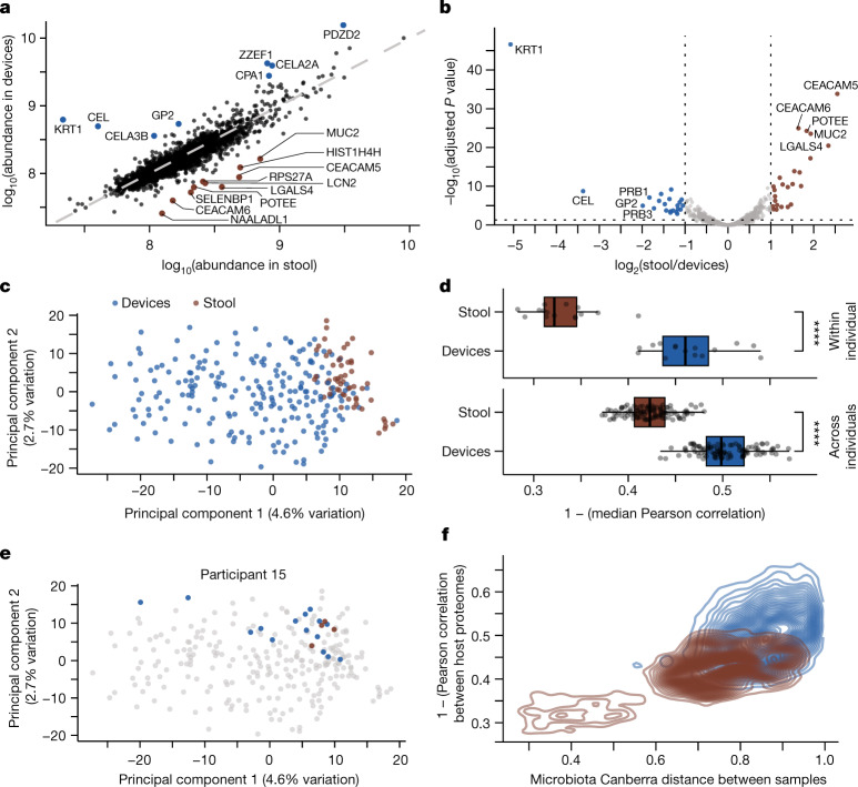
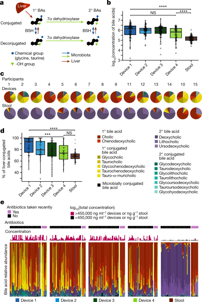
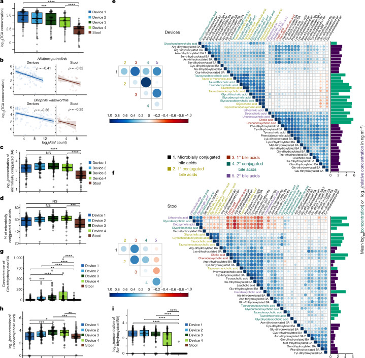
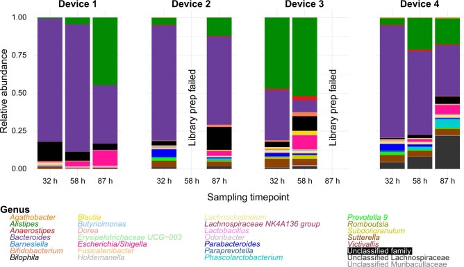
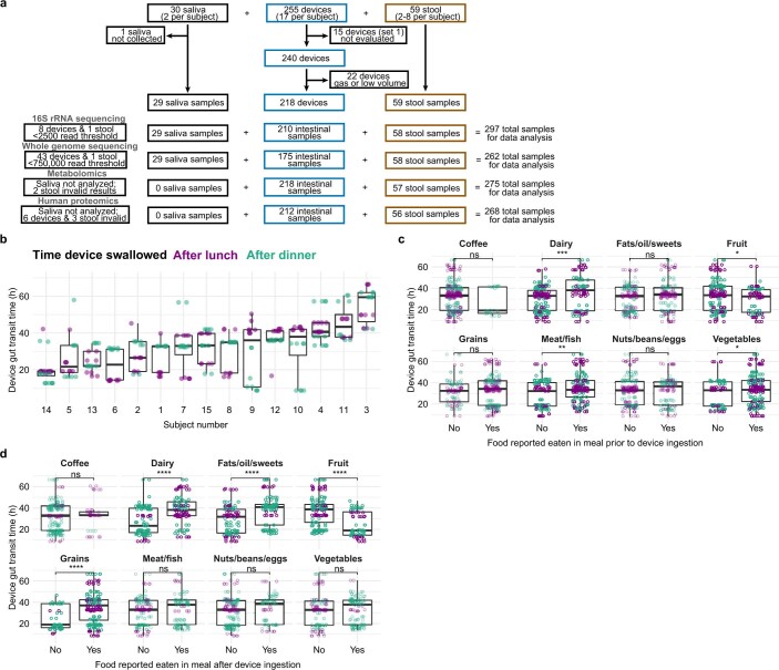
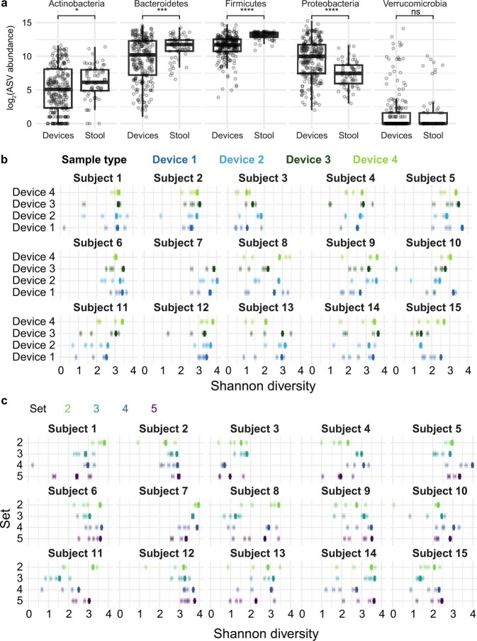
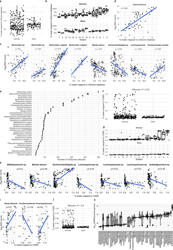
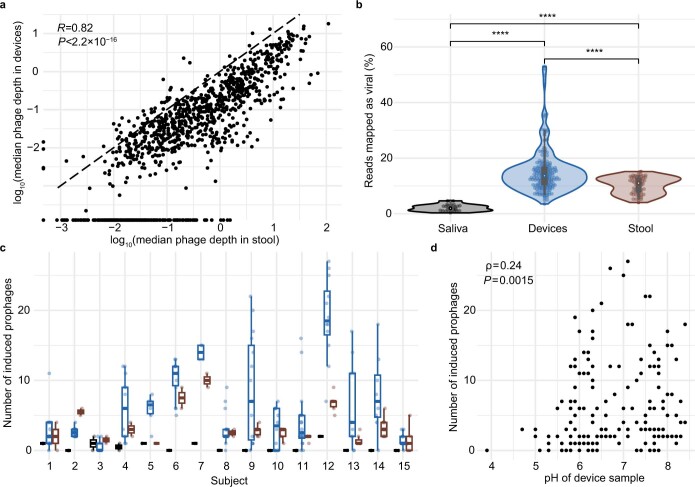
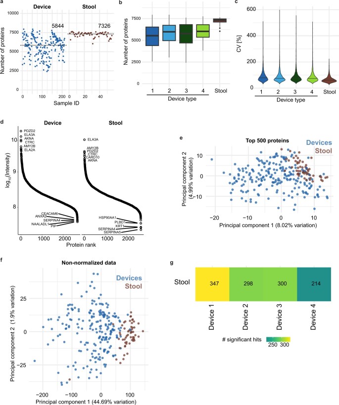
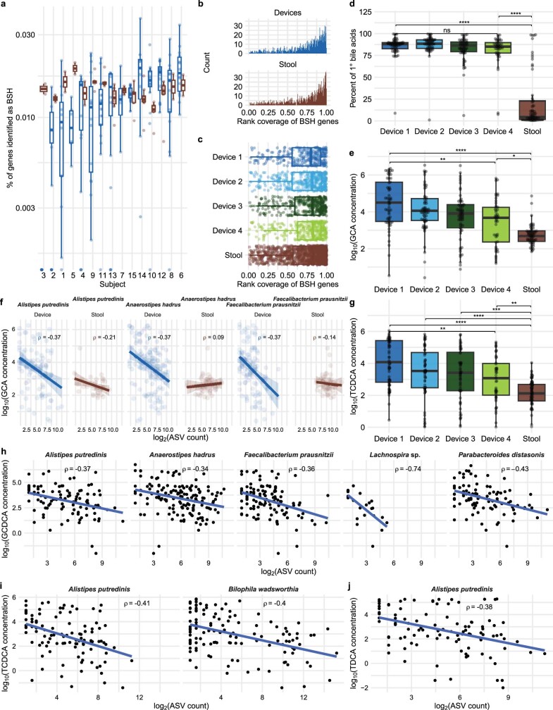
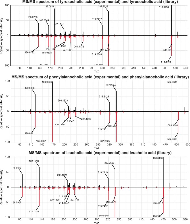
The spatiotemporal structure of the human microbiome^1,2, proteome³ and metabolome^4,5 reflects and determines regional intestinal physiology and may have implications for disease⁶. Yet, little is known about the distribution of microorganisms, their environment and their biochemical activity in the gut because of reliance on stool samples and limited access to only some regions of the gut using endoscopy in fasting or sedated individuals⁷. To address these deficiencies, we developed an ingestible device that collects samples from multiple regions of the human intestinal tract during normal digestion. Collection of 240 intestinal samples from 15 healthy individuals using the device and subsequent multi-omics analyses identified significant differences between bacteria, phages, host proteins and metabolites in the intestines versus stool. Certain microbial taxa were differentially enriched and prophage induction was more prevalent in the intestines than in stool. The host proteome and bile acid profiles varied along the intestines and were highly distinct from those of stool. Correlations between gradients in bile acid concentrations and microbial abundance predicted species that altered the bile acid pool through deconjugation. Furthermore, microbially conjugated bile acid concentrations exhibited amino acid-dependent trends that were not apparent in stool. Overall, non-invasive, longitudinal profiling of microorganisms, proteins and bile acids along the intestinal tract under physiological conditions can help elucidate the roles of the gut microbiome and metabolome in human physiology and disease.

Fig. 1. Devices enable longitudinal sampling of the human intestine.

a, Overview of the intended sampling locations (top) of the four device types in packaged form for ingestion (middle) and as full collection bladders containing intestinal samples after retrieval from stool (bottom). A US dime is included for scale. Top right, the device contains a folded bladder capped with a one-way valve within a capsule with an enteric coating, which dissolves once the designated pH has been reached, enabling the bladder to unfold and draw in up to 400 µl of luminal fluid. b, Timeline for the collection of saliva, intestinal and stool samples from 15 healthy adults. Set 1 devices were not used for analyses. c, Family-level relative abundance for each sample by participant and location (n = 268). The colour of the ASV indicates the phylum, and the gradient of a given colour represents different families within the phylum. Only 16S rRNA gene ASVs with ≥3 reads in ≥5% of device and stool samples were used (n = 399 ASVs). d, The pH of the contents in devices designed to open at locations spanning the proximal to distal intestinal tract exhibited the expected increasing trend. Points represent individual devices (n = 218). P values from top to bottom: 0.018, 1.1 × 10^–4, 5.5 × 10⁻⁵, 8.6 × 10⁻⁸, 1 and 0.19. Boxplots show the median value and the first and third quartiles. NS, not significant; **P ≤ 0.01, ****P ≤ 0.0001, Bonferroni-adjusted two-sided Wilcoxon rank-sum test. e, PCoA based on Canberra distance between microbial communities (n = 297). Read counts were log₂ transformed. Each point represents an individual sample and is coloured by the sample type (stool, saliva and device types 1–4). Filled squares and triangles identify two outlier participants (10 and 15) who had taken oral antibiotics in the 5 months before intestinal sampling. Only 16S rRNA gene ASVs with ≥3 reads in ≥5% of samples (including saliva) were used (n = 455 ASVs). f, ASVs with log₂(fold change) > 0.75 between devices and stool that were significantly differentially abundant (n = 28 ASVs across n = 268 analysed samples; limma-voom was used to calculate differential expression after size factors were estimated and normalized using DESeq2; P < 0.05, Benjamini–Hochberg correction).

Fig. 2. Microbiota variation across device types suggests patchy structure.

a, Microbiota composition varied significantly more between intestinal samples than between stool samples (P = 1.5 × 10⁻⁷ within participants and P = 2.3 × 10⁻²² across participants) or between saliva samples (P = 1.5 × 10⁻⁷ within participants and P = 3.5 × 10⁻³⁵ across participants). Top, each point is the mean pairwise Canberra distance between all samples for a participant (n = 14, 15 and 14 for stool, devices and saliva, respectively). Bottom, each point is the mean of all pairwise comparisons between all samples from any two participants (n = 105, 105 and 105 for stool, devices and saliva, respectively). b, Combinations of spatial, temporal and technical (n = 15 each) variability in the microbiota composition of intestinal samples (gray) were higher than in technical replicates (n = 8; light brown) in which one participant swallowed four of the same device type simultaneously (the participant did so twice for each of the four device types). Each point represents the mean pairwise Canberra distance between intestinal samples from the same participant. Microbial communities from devices of the same type ingested at the same time were more similar than those from devices of the same type ingested at different times, although this difference was not statistically robust (P = 0.058) given the small number of observations. c, Devices were more likely to be dominated by a single ASV as compared with stool or saliva. Each point is a single sample (n = 29 for saliva, n = 56, 54, 55 and 45 for device types 1–4, respectively, and n = 58 for stool). d, The Shannon diversity of saliva and stool samples was higher than that of intestinal samples (saliva to device type 1, P = 5.3 × 10⁻⁷; device type 4 to stool, P = 2.9 × 10⁻⁹). Each point is a single sample (n = 29 for saliva, n = 56, 54, 55 and 45 for device types 1–4, respectively, and n = 58 for stool). Boxplots show the median value and the first and third quartiles. *P ≤ 0.05, ****P ≤ 0.0001, Bonferroni-adjusted two-sided Wilcoxon rank-sum test. Canberra distances for a,b were computed from log₂-transformed read counts of 16S rRNA gene ASVs with read count ≥3 in ≥5% of samples (including all repeatability samples) (n = 446).

Fig. 3. Prophage induction is more frequent in the intestines than in stool.

a, Stool and intestinal samples share most vOTUs. Only vOTUs at a depth of ≥1.0 were included. b, PCoA based on Canberra distance between profiles of vOTUs detected in samples coloured on the basis of sample type. c, Intestinal samples contained significantly higher numbers of induced prophages than stool (P = 0.026) or saliva (P = 2.5 × 10⁻¹¹) samples. n = 29, 172 and 58 for saliva, intestinal and stool samples, respectively. P values are from a two-sided Wilcoxon rank-sum test. Density boxplots show the median value and the first and third quartiles. d, Most prophages induced in stool samples are also induced in the intestines, but many other induced prophages are unique to intestinal samples.

Fig. 4. Human protein abundance differs between stool and intestinal samples.

a, Median log₁₀(abundance) of human proteins in stool samples (n = 56) compared with intestinal samples (n = 212). b, log₂(fold change) of each protein abundance in stool relative to intestinal samples. A two-sample modified t-test with Benjamini–Hochberg correction was used. Proteins with absolute log₂(fold change) > 1 and P < 0.05 are coloured on the basis of sample type and enrichment. c, PCA of normalized human protein abundance shows separation between intestinal and stool samples (n = 212 and 56, respectively). d, Human proteome composition varies significantly more between intestinal samples (n = 212) than between stool samples (n = 56), both within (top) and across (bottom) participants. Top, each circle is the median Pearson correlation coefficient of all sample pairs for a given participant. Bottom, each circle is the median of all correlation coefficients between all pairs of samples from any two participants (n = 105 for each intestinal and stool sample). ****P ≤ 0.0001, Bonferroni-corrected two-tailed Wilcoxon rank-sum test. e, PCA from c highlighting the clustering of intestinal and stool samples from participant 15 (n = 15 and 4, respectively). f, Canberra distance between microbiota compositions was higher in samples with less similar human proteomes for all sample pairs of a given type (n = 20,706 pairwise comparisons for devices, n = 1,485 pairwise comparisons for stool).

Fig. 5. Devices capture different bile acid profiles along the intestinal tract compared with stool.

a, Schematic of bile acid (BA) modifications by the liver and microbiota. The liver releases bile acids conjugated with glycine or taurine. Dehydroxylation by gut microorganisms converts primary (1°) to secondary (2°) bile acids. Microbial BSHs deconjugate amino acids from bile salts. b, The total concentration of all bile acids decreases along the intestinal tract (device type 1 to stool, P = 2.0 × 10⁻⁹; device type 4 to stool, P = 5.6 × 10⁻⁴; device type 1 to 4, P = 0.18). Shown are log₁₀-transformed concentrations for intestinal (n = 58, 56, 57 and 47 for device types 1–4, respectively) or stool (n = 57) samples. c, The mean relative concentration of all bile acids for each participant in devices and stool. In all but two participants (10 and 15), DCA and LCA dominated the stool, but not the intestines. d, The percentage of liver-conjugated bile acids decreases significantly along the intestinal tract (device type 1 to stool, P = 2.2 × 10⁻¹⁰; device type 4 to stool, P = 0.20; device type 1 to 4, P = 3.2 × 10⁻⁴; n = 58, 56, 57 and 47 for device types 1–4, respectively, and n = 57 for stool samples). e, Relative abundance of bile acids for each sample arranged by device type. Participants are ordered 1–9, 11–14, 10, 15 within each device type. Antibiotic usage and log₁₀(total concentration of bile acids) in the sample are also shown. Boxplots show the median and first and third quartiles. ***P ≤ 0.001, ****P ≤ 0.0001, Bonferroni-corrected two-sided Wilcoxon rank-sum test. Concentrations are in units of ng ml^–1 or ng g^–1 for devices and stool, respectively.

Fig. 6. Bile acid relationships in intestines and stool.

a, TCA concentration decreases along the intestinal tract. Shown are log₁₀-transformed concentrations. Device type 1 to 4, P = 10⁻³; device type 1 to stool, P = 6.2 × 10⁻¹⁴; device type 4 to stool, P = 5.5 × 10⁻⁷. b, log₂(read count) of an A. putredinis ASV and a B. wadsworthia ASV was negatively correlated (P = 0.0020 and P = 0.0042, respectively) with TCA concentration. Correlations were weaker in stool samples (P = 0.36 and P = 0.56, respectively). Correlations are Spearman correlations with Benjamini–Hochberg correction. Only ASVs with P < 0.01 after correction in devices are shown. Points are individual intestinal (n = 210) or stool (n = 56) samples for which both 16S rRNA sequencing and metabolomics data were available. c, The concentration of microbially conjugated bile acids is significantly higher in intestinal samples than in stool samples. The concentration did not differ significantly across device types. Device type 1 to 4, P = 1; device type 1 to stool, P = 3.5 × 10⁻⁶; device type 4 to stool, P = 1.6 × 10⁻⁶. d, The percentage of microbially conjugated bile acids increases along the intestinal tract and was significantly higher in intestinal samples than in stool. Device type 1 to 4, P = 0.40; device type 1 to stool, P = 0.23; device type 4 to stool, P = 8.0 × 10⁻⁴. e,f, Correlations between bile acid profiles differ between intestinal (e) and stool (f) samples. Shown are Pearson correlation coefficients using log₁₀-transformed concentrations. Horizontal bars show the mean absolute concentration (green) or relative concentration (purple) (Methods). Bile acid ordering was determined by hierarchical clustering. Insets show the Pearson correlation coefficient for aggregated classes. g–i, Concentration of the respective bile acid across devices and stool. P values from top to bottom for g: 4.3 × 10⁻⁹, 7.5 × 10⁻⁹, 5.1 × 10⁻⁷, 7.0 × 10⁻³, 1.8 × 10⁻⁴ and 6.5 × 10⁻⁴. P values from top to bottom for h: 0.001, 5.8 × 10⁻⁵, 0.023 and 1.4 × 10⁻⁴. P values from top to bottom for i: 5.9 × 10⁻¹³, 1.5 × 10⁻¹⁶, 8.5 × 10⁻²⁰ and 6.2 × 10⁻¹⁹. All boxplots show the median and first and third quartiles. Points are individual intestinal (n = 58, 56, 57 and 47 for device types 1–4, respectively) or stool (n = 57) samples, unless otherwise indicated. Concentrations in ng ml^–1 (intestinal) or ng g^–1 (stool). *P ≤ 0.1, **P ≤ 0.01, ***P ≤ 0.001, ****P ≤ 0.0001, Bonferroni-corrected two-sided Wilcoxon rank-sum test.

Extended Data Fig. 1. Changes in intestinal microbiota composition during sample incubation.

Devices were collected from a bowel movement of a single subject 32 h after ingestion and placed immediately into an anaerobic chamber at 37 °C. Samples were collected from each device immediately (32 h) and again at 58 h and 87 h. Samples were then prepared for 16S rRNA gene sequencing. Genus-level relative abundance is shown for all ASVs with read count ≥15 in any single sample.

Extended Data Fig. 2. Total gut transit time of devices varied across subjects and diets.

a) Subjects (n = 15) enrolled in the study ingested a total of 17 intestinal sampling devices each (set 1 consisted of a single device used as a safety test to ensure safe passage through the intestines). Subjects were also asked to provide two saliva samples and collect stool until all intestinal sampling devices were retrieved. Between two and eight stool samples from each subject were used for analysis. b) Device (n = 240) gut transit time was variable across subjects. Some subjects displayed differences in transit time dependent on the time of day the device was ingested. c) Device gut transit time varied according to certain types of food consumed in the meal prior to device ingestion (i.e., the food with which the devices presumably transited into the small intestines). P-values from left to right, top to bottom: 0.18, 0.00091, 0.24, 0.17, 0.29, 0.0049, 0.57, and 0.27. d) Device gut transit time varied according to the type of food consumed in the meal after devices were swallowed (i.e., the food that likely influenced gut motility while devices were passing through the large intestines). P-values from left to right, top to bottom: 0.68, 1.4 × 10⁻⁷, 1.1 × 10⁻⁷, 7.6 × 10⁻¹¹, 7 × 10⁻⁷, 0.49, 0.25, and 0.3. Boxplots show the median and 1^st and 3^rd quartiles. Each dot is a device sample (b–d; n = 60 each for device types 1–4). ns: not significant, *: P ≤ 0.05, **: P ≤ 0.01, ***: P ≤ 0.001, ****: P ≤ 0.0001, Bonferroni-corrected two-sided Wilcoxon rank-sum test. Alcohol consumption and diet contents were not restricted. Subjects swallowed devices 3 h after lunch and dinner and were instructed not to consume any additional foods for at least 2 h after swallowing devices.

Extended Data Fig. 3. Diversity in phylum abundances and alpha and gamma diversity implicate a temporally and spatially heterogeneous intestinal tract.

a) Summed log₂(read count) at the phylum level are shown for each sample by location. P-values from left to right: 0.57, 0.0035, 2.4 × 10⁻¹⁵, 5.7 × 10⁻⁷, and 0.83. ASVs that did not have read count ≥3 in 5% of samples were ignored. Boxplots show the median and 1^st and 3^rd quartiles. Each dot represents a sample (n = 210 and 58 for devices and stool, respectively). ns: not significant, *: P ≤ 0.05, **: P ≤ 0.01, ***: P ≤ 0.001, ****: P ≤ 0.0001, Bonferroni-corrected two-sided Wilcoxon rank-sum test. b, c) The Shannon diversity of individual devices (n = 210 devices; alpha diversity, lighter points) was generally lower than that collectively of all devices from a single set (gamma diversity, bold points), indicating high spatial variation. Each subject (#1–#15) is shown separately. To ensure equal read depths for accurate comparisons, all intestinal samples were rarefied to the minimum sequencing depth of any device from that subject. Mean values and 95% confidence intervals for alpha and gamma diversity estimates were obtained by repeating the rarefaction procedure 1000 times.

Extended Data Fig. 4. Growing cells recovered from devices collectively displayed a wide range of morphologies.

a) A 2-µL sample was acquired from a single device and spotted onto an agarose pad with BHI medium. After 4 h of time-lapse imaging, growing cells displayed a wide range of morphological features, as highlighted by white arrows: 1. regular rods; 2. small rods; 3. wide rods; 4. branching; and 5. long/filamentous rods. Along with the sample shown, 3 other samples from devices ingested at the same time were imaged, and similar results were observed. b) Occasional human cells (white arrow) were observed during imaging.

Extended Data Fig. 5. Percent of reads mapping to CAZymes and antimicrobial resistance genes vary across the intestinal tract and are driven by distinct taxa.

a) The percent of reads that mapped to a database of CAZymes (Methods) was determined using metagenomic sequencing of each sample. b) Data from (a) separated by subject. c) In intestinal samples, the log₂(read count) of eight ASVs was positively correlated (Spearman) with the percent of reads that mapped to the CAZyme database. Only ASVs with P < 0.001 are shown. P-values from left to right, top to bottom: 1.8 × 10⁻⁶, 7.2 × 10⁻⁴, 1.1 × 10⁻²⁴, 3.7 × 10⁻⁴, 3.7 × 10⁻⁴, 2.6 × 10⁻⁵, 3.7 × 10⁻⁴, and 3.7 × 10⁻⁴. d) The log₂(ASV read count summed over family members) of the Bacteroidaceae family was significantly correlated (Spearman; P = 6.4 × 10⁻⁷) with the percent of reads from stool samples that mapped to the CAZyme database. No other families had P < 0.01. e) The number of CAZymes identified in strains isolated from the intestinal tract of subject 1, organized by species. Each circle represents a single strain, and horizontal lines (mostly hidden by the circles) represent the median. f) The percent of reads that mapped to a database of AMR genes (CARD, Methods) was determined using metagenomics sequencing of each sample and was higher in devices compared with stool (P = 0.03). g) Data from (f) separated by subject. h) In intestinal samples, the log₂(read count) of two ASVs was positively correlated (Spearman) with the percent of reads that mapped to CARD. Only ASVs with P < 0.001 are shown. P-values from left to right, top to bottom: 5.7 × 10⁻⁸, 1.5 × 10⁻⁴, 4.1 × 10⁻⁷, 2.5 × 10⁻⁴, 6.4 × 10⁻⁵, 2.0 × 10⁻⁸, and 2.1 × 10⁻⁴. i) In stool samples, the log₂(ASV read count summed over family members) of families was significantly correlated (Spearman; P = 5.7×10⁻⁵, 1.5 × 10⁻³, and 7.1 × 10⁻⁴) with the percent of reads that mapped to a database of AMR genes. No other families had P < 0.001. j) The percent of reads that mapped to CARD ignoring all efflux pumps was similar between devices and stool (P = 0.8). k) log₁₀(ratio of the number of AMR genes to bacterial genes) detected in each MAG, aggregated by family-level taxonomic assignment. Only MAGs with completion >75% and contamination <10% were included. In (a–d and f–j), each dot is a sample (n = 175 for devices and n = 58 for stool). All P-values reported are after Benjamini-Hochberg correction. Boxplots show the median and 1^st and 3^rd quartiles.

Extended Data Fig. 6. Intestinal samples have higher bacteriophage load.

a) The median sequencing depth of vOTUs (n = 1343) in intestinal samples was highly correlated with depth in stool samples (Pearson; P < 2.2 × 10⁻¹⁶). 481 vOTUs appeared in less than half of the intestinal samples and hence the median was 0 (represented as 10⁻⁴). b) Intestinal samples had significantly higher read fraction mapping to vOTUs. n = 29, 172, and 58 for saliva, intestinal, and stool samples, respectively. P-values are from two-tailed Student’s t-tests. P-values from top to bottom, left to right: 4.7 × 10⁻¹⁴, 2.2 × 10⁻¹⁶, 2.3 × 10⁻⁷. c) The number of induced prophages was generally higher in intestinal samples across subjects and was lowest in saliva samples. d) pH was correlated with the number of induced prophages in intestinal samples (Spearman; P = 0.0015).

Extended Data Fig. 7. Comparison of the human proteome in intestinal versus stool samples.

a) The number of host-associated proteins detected in each sample, colored by location (intestinal versus stool). Dotted line and number represent the mean. b) The number of host-associated proteins detected across samples from each device type and stool. Boxplot shows the median and 1^st and 3^rd quartiles. c) The distribution of coefficient of variation (CV) for all detected host proteins across device types and stool samples. d) Proteins were ranked based on mean log₁₀(intensity) for intestinal and stool samples. The six most and five least abundant proteins are labelled for each location. e) A principal component analysis of the normalized abundance of the 500 most abundant host-associated proteins. Results are similar to Fig. 4c. Points are colored based on location of sample (intestinal versus stool). f) A principal component analysis of the non-normalized abundance of all host-associated proteins found in each sample. Results are qualitatively similar to Fig. 4c and e. Points are colored based on location of sample (intestinal versus stool). g) The number of host-associated proteins with significantly different abundance between stool and each device type based on a 5% false discovery rate (FDR). All panels used n = 56 stool and n = 212 device samples for analysis. In (b,c,g), n = 56 type 1, n = 54 type 2, n = 56 type 3, and n = 46 type 4 device samples were used.

Extended Data Fig. 8. Microbial bile salt hydrolase genes exhibited similar abundance and diversity in intestinal and stool samples despite differences in conjugated bile acids along the intestinal tract.

a) Open reading frames identified as bile salt (cholylglycine) hydrolase (BSH) enzymes via a hidden Markov model (HMM) search, normalized by the total number of open reading frames detected in the sample. b) The distribution of rank coverage of bsh genes was similar between intestinal and stool samples. c) Rank coverages of bsh genes in devices of each type and in stool are similar. (all P > 0.90). d) Percentage of primary (hydroxylated) bile acids was similar across device types and was lower in stool compared with intestinal samples (top to bottom: P = 3.7 × 10⁻¹³, 1.3 × 10⁻¹⁰, and 0.91). e) Glycocholic acid (GCA) concentration decreased along the intestinal tract (top to bottom: P = 1.6 × 10⁻¹², 0.035, and 0.003). f) The log₂(ASV count) of Alistipes putredinis, Anaerostipes hadrus, and Bilophila wadsworthia was negatively correlated (Spearman; P = 0.0068, 0.0004, and 0.0068 in devices and P = 0.63, 0.84, and 0.70 in stool, respectively) with log₁₀(GCA concentration). Only ASVs with P < 0.01 after a Benjamini-Hochberg correction in device samples are shown. g) Taurochenodeoxycholic acid (TCDCA) concentration decreased along the intestinal tract (top to bottom: P = 0.0070, 1.9 × 10⁻⁴, 4.2 × 10⁻⁶, 1.5 × 10⁻¹⁰, and 0.0020). h) log₂(ASV read count) of Alistipes putredinis and Bilophila wadsworthia in devices was negatively correlated (Spearman; P = 2.5 × 10⁻⁵ and 3.3 × 10⁻⁷, respectively) with log₁₀(TCDCA concentration). Only ASVs with P < 0.01 after a Benjamini-Hochberg correction in device samples are shown. i) log₂(ASV read count) of Bilophila wadsworthia in devices was negatively correlated (Spearman; P = 2.4 × 10⁻⁵) with log₁₀(concentration of taurodeoxycholic acid (TDCA)). Only ASVs with P < 0.01 after a Benjamini-Hochberg correction in device samples are shown. In (a–c), n = 175 device and n = 58 stool samples were used for analysis. In (d–h), n = 210 device samples and n = 56 stool samples were used for analysis. All boxplots show the median and 1^st and 3^rd quartiles. ns: not significant, ****: P ≤ 0.0001, Bonferroni-corrected two-sided Wilcoxon rank-sum test. Bile acids shown are log₁₀-transformed concentrations in units of ng/mL or ng/g for intestinal or stool samples, respectively.

Extended Data Fig. 9. Microbially conjugated bile acid identification.

Head-to-tail matches of experimental (top) to library (bottom) spectra from bile acids conjugated to tyrosine, phenylalanine, and leucine.

References

1. Hillman ET, Lu H, Yao T, Nakatsu CH. Microbial ecology along the gastrointestinal tract. Microbes Environ. 2017;32:300–313. doi: 10.1264/jsme2.ME17017. - DOI - PMC - PubMed
1. Tabula Sapiens C, et al. The Tabula Sapiens: a multiple-organ, single-cell transcriptomic atlas of humans. Science. 2022;376:eabl4896. doi: 10.1126/science.abl4896. - DOI - PMC - PubMed
1. Lichtman JS, et al. The effect of microbial colonization on the host proteome varies by gastrointestinal location. ISME J. 2016;10:1170–1181. doi: 10.1038/ismej.2015.187. - DOI - PMC - PubMed
1. Chiang JY. Bile acid metabolism and signaling. Compr. Physiol. 2013;3:1191–1212. doi: 10.1002/cphy.c120023. - DOI - PMC - PubMed
1. Zhou H, Hylemon PB. Bile acids are nutrient signaling hormones. Steroids. 2014;86:62–68. doi: 10.1016/j.steroids.2014.04.016. - DOI - PMC - PubMed
Publication types