. 2023 May;617(7960):312-324.
doi: 10.1038/s41586-023-05896-x. Epub 2023 May 10.

A draft human pangenome reference

Wen-Wei Liao #  1   2   3 Mobin Asri #  4 Jana Ebler #  5   6 Daniel Doerr  5   6 Marina Haukness  4 Glenn Hickey  4 Shuangjia Lu  1   2 Julian K Lucas  4 Jean Monlong  4 Haley J Abel  7 Silvia Buonaiuto  8 Xian H Chang  4 Haoyu Cheng  9   10 Justin Chu  9 Vincenza Colonna  8   11 Jordan M Eizenga  4 Xiaowen Feng  9   10 Christian Fischer  11 Robert S Fulton  12   13 Shilpa Garg  14 Cristian Groza  15 Andrea Guarracino  11   16 William T Harvey  17 Simon Heumos  18   19 Kerstin Howe  20 Miten Jain  21 Tsung-Yu Lu  22 Charles Markello  4 Fergal J Martin  23 Matthew W Mitchell  24 Katherine M Munson  17 Moses Njagi Mwaniki  25 Adam M Novak  4 Hugh E Olsen  4 Trevor Pesout  4 David Porubsky  17 Pjotr Prins  11 Jonas A Sibbesen  26 Jouni Sirén  4 Chad Tomlinson  12 Flavia Villani  11 Mitchell R Vollger  17   27 Lucinda L Antonacci-Fulton  12 Gunjan Baid  28 Carl A Baker  17 Anastasiya Belyaeva  28 Konstantinos Billis  23 Andrew Carroll  28 Pi-Chuan Chang  28 Sarah Cody  12 Daniel E Cook  28 Robert M Cook-Deegan  29 Omar E Cornejo  30 Mark Diekhans  4 Peter Ebert  5   6   31 Susan Fairley  23 Olivier Fedrigo  32 Adam L Felsenfeld  33 Giulio Formenti  32 Adam Frankish  23 Yan Gao  34 Nanibaa' A Garrison  35   36   37 Carlos Garcia Giron  23 Richard E Green  38   39 Leanne Haggerty  23 Kendra Hoekzema  17 Thibaut Hourlier  23 Hanlee P Ji  40 Eimear E Kenny  41 Barbara A Koenig  42 Alexey Kolesnikov  28 Jan O Korbel  23   43 Jennifer Kordosky  17 Sergey Koren  44 HoJoon Lee  40 Alexandra P Lewis  17 Hugo Magalhães  5   6 Santiago Marco-Sola  45   46 Pierre Marijon  5   6 Ann McCartney  44 Jennifer McDaniel  47 Jacquelyn Mountcastle  32 Maria Nattestad  28 Sergey Nurk  44 Nathan D Olson  47 Alice B Popejoy  48 Daniela Puiu  49 Mikko Rautiainen  44 Allison A Regier  12 Arang Rhie  44 Samuel Sacco  30 Ashley D Sanders  50 Valerie A Schneider  51 Baergen I Schultz  33 Kishwar Shafin  28 Michael W Smith  33 Heidi J Sofia  33 Ahmad N Abou Tayoun  52   53 Françoise Thibaud-Nissen  51 Francesca Floriana Tricomi  23 Justin Wagner  47 Brian Walenz  44 Jonathan M D Wood  20 Aleksey V Zimin  49   54 Guillaume Bourque  55   56   57 Mark J P Chaisson  22 Paul Flicek  23 Adam M Phillippy  44 Justin M Zook  47 Evan E Eichler  17   58 David Haussler  4   58 Ting Wang  12   13 Erich D Jarvis  32   58   59 Karen H Miga  4 Erik Garrison  60 Tobias Marschall  61   62 Ira M Hall  63   64 Heng Li  65   66 Benedict Paten  67
Affiliations

A draft human pangenome reference

Wen-Wei Liao et al. Nature. 2023 May.

Abstract

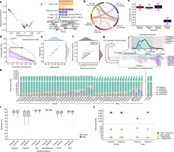
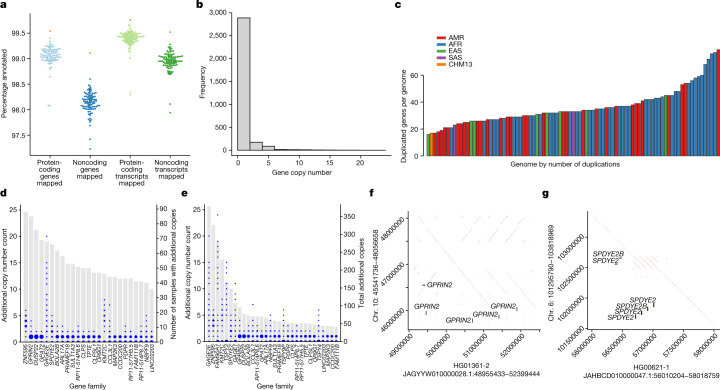
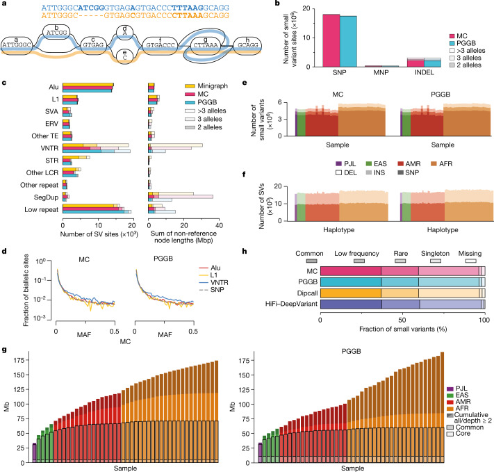
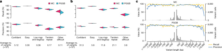
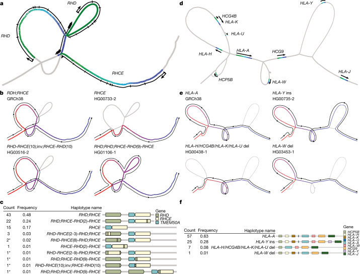
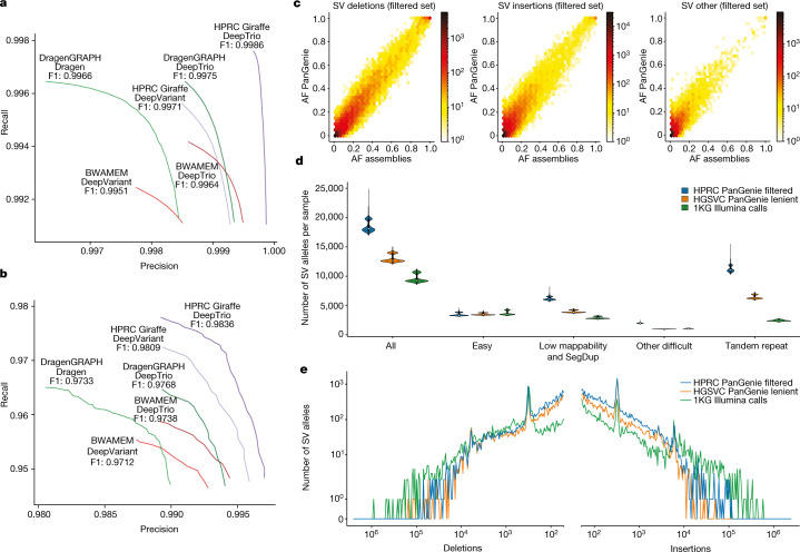
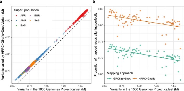
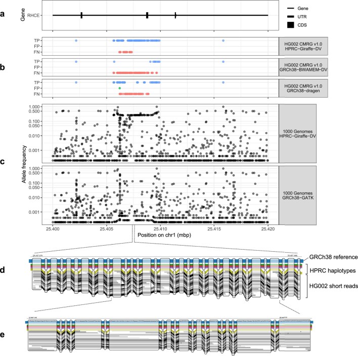
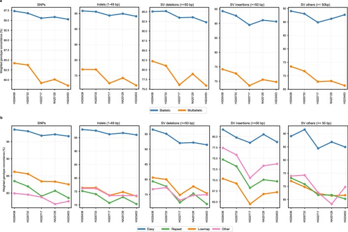
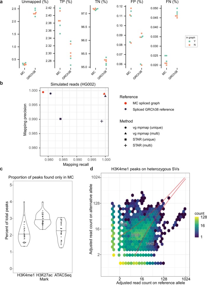
Here the Human Pangenome Reference Consortium presents a first draft of the human pangenome reference. The pangenome contains 47 phased, diploid assemblies from a cohort of genetically diverse individuals1. These assemblies cover more than 99% of the expected sequence in each genome and are more than 99% accurate at the structural and base pair levels. Based on alignments of the assemblies, we generate a draft pangenome that captures known variants and haplotypes and reveals new alleles at structurally complex loci. We also add 119 million base pairs of euchromatic polymorphic sequences and 1,115 gene duplications relative to the existing reference GRCh38. Roughly 90 million of the additional base pairs are derived from structural variation. Using our draft pangenome to analyse short-read data reduced small variant discovery errors by 34% and increased the number of structural variants detected per haplotype by 104% compared with GRCh38-based workflows, which enabled the typing of the vast majority of structural variant alleles per sample.


Conflict of interest statement

E.E.E. is a scientific advisory board (SAB) member of Variant Bio. P.F is a member of the SABs of Fabric Genomics and Eagle Genomics. E.E.K. is a member of the SAB of Encompass Biosciences, Foresite Labs and Galateo Bio and has received personal fees from Regeneron Pharmaceuticals, 23&Me and Illumina. A.B., A.C., P.-C.C., D.E.C., G.Baid, A.K., M.N. and K.S. are employees of Google and own Alphabet stock as part of the standard compensation package.

Figures

Fig. 1
Fig. 1. Presenting 47 accurate and near-complete diverse diploid human genome assemblies.
a, Selecting the HPRC samples. Left, the first two principal components of 1KG samples showing HPRC (triangles) samples, excluding HG002, HG005 and NA21309. Right, summary of the HPRC sample subpopulations (three letter abbreviations) on a map of Earth as defined by the 1KG. ACB, African Caribbean in Barbados; ASW, African Ancestry in Southwest US; CHS, Han Chinese South; CLM, Colombian in Medellin, Colombia; ESN, Esan in Nigeria; GWD, Gambian in Western Division; KHV, Kinh in Ho Chi Minh City, Vietnam; MKK, Maasai in Kinyawa, Kenya; MSL, Mende in Sierra Leone; PEL, Peruvian in Lima, Peru; PJL, Punjabi in Lahore, Pakistan; PUR, Puerto Rican in Puerto Rico; YRI, Yoruba in Ibadan, Nigeria. b, Interchromosomal joins between acrocentric chromosome short arms. Red, the join is on the same strand; blue, otherwise. c, Total assembled sequence per haploid phased assembly. d, Assembly contiguity shown as a NGx plot. T2T-CHM13 and GRCh38 contigs are included for comparison. e, Assembly QVs showing the base-level accuracy of the maternal and paternal assembly for each sample. f, Yak-reported phasing accuracy showing the switch error percentage versus Hamming error percentage. g, Flagger read-based assembly evaluation pipeline. Coverage is calculated across the genome and a mixture model is fit to account for reliably assembled haploid sequence and various classes of unreliably assembled sequence. For each coverage block, a label is assigned according to the most probable mixture component to which it belongs: erroneous, falsely duplicated, (reliable) haploid, collapsed, and unknown. h, Reliability of the 47 HPRC assemblies using read mapping. For each sample, the left bar is the paternal and the right bar is the maternal haplotype. Regions flagged as haploid are reliable (green), constituting more than 99% on average of each assembly. The y axis is broken to show the dominance of the reliable haploid component and the stratification of the unreliable blocks. i, Assembly reliability of six types of repeats. AlphaSat, alpha satellites; HSat2/3, human satellites 2 and 3. j, Completeness of the HPRC assemblies relative to T2T-CHM13. The number of reference bases covered by none, by one, by two or by more than two alignments are included.
Fig. 2
Fig. 2. Transcriptome annotation of the assemblies.
a, Ensembl mapping pipeline results. Percentages of protein-coding and noncoding genes and transcripts annotated from the reference set in each of the HPRC assemblies. Orange points represent T2T-CHM13 for comparison. b, Frequency of gene copy number. Individual genes may have separate copy number states among genomes, and the frequency reflects 3,210 observed copy number changes among the HPRC genomes. c, Number of distinct duplicated genes or gene families per phased assembly relative to the number of duplicated genes annotated in GRCh38 (n = 152). The GRCh38 gene duplications reflect families of duplicated genes, whereas the counts in other genomes reflect gene duplication polymorphisms. The assemblies are colour coded according to their population of origin. d, The top 25 most commonly CNV genes or gene families in the HPRC assemblies out of all 1,115 duplicated genes, ordered by the number of samples with additional copies relative to GRCh38. Grey bars, the number of samples with additional copies. Blue circles, the number of additional copies per sample, with the size of the circle proportional to the number of samples. e, The top 30 most individually copied CNV genes or gene families in the HPRC assemblies, ordered by total number of additional copies observed. Blue circles, the number of additional copies per sample. Grey bars, the total number of additional copies summed over the samples. f, Dotplot illustrating haplotype-resolved GPRIN2 gains in the HG01361 assembly relative to GRCh38. g, Dotplot illustrating SPDYE2SPDYE2B haplotype resolved gains within a tandem duplication cluster of the HG00621 assembly relative to GRCh38.
Fig. 3
Fig. 3. Pangenome graphs represent diverse variation.
a, A pangenome variation graph comprising two elements: a sequence graph, the nodes of which represent oriented DNA strings and bidirected edges represent the connectivity relationships; and embedded haplotype paths (coloured lines) that represent the individual assemblies. b, Small variant sites in pangenome graphs stratified by the variant type and by the number of alleles at each site. MNP, multinucleotide polymorphism. c, SV sites in the pangenome graphs stratified by repeat class and by the number of alleles at each site. Other TE, a site involving mixed classes of transposable elements (TEs). VNTR, variable-number tandem repeat, a tandem repeat with the unit motif length ≥7 bp. STR, short tandem repeat, a tandem repeat with the unit motif length ≤6 bp. Other LCR, low-complexity regions with mixed VNTR and STR and low-complexity regions without a clear VNTR or STR pattern. Other repeat, a site involving mixed classes of repeats. SegDup, segmental duplication. Low repeat, a small fraction of the longest allele in a site involving repeats. d, Pangenome minor AF (MAF) spectrum for biallelic SNP, VNTR, L1 and Alu variants in the MC and PGGB graphs. e,f, Number of autosomal small variants per sample (e) and SVs per haplotype (f) in the pangenome. Variants were restricted to the Dipcall-confident regions. Samples are organized by 1KG populations. g, Pangenome growth curves for MC (left) and PGGB (right). Depth measures how often a segment is contained in any haplotype sequence, whereby core is present in ≥95% of haplotypes, common is ≥5%. h, Small variants in the GIAB (v.3.0) ‘easy’ regions annotated with AFs from gnomAD (v.3.1.2).
Fig. 4
Fig. 4. Pangenome graph evaluation.
a,b, Precision and recall of autosomal small variants (a) and SVs (b) in the pangenomes relative to consensus variant sets. Small variants are compared to HiFi–DeepVariant calls. SVs are compared to the consensus of six reference-based SV callers (Methods). Comparisons are restricted to the Dipcall-confident regions and then stratified by the GIAB (v.3.0) genomic context. c, Average SV precision, recall and frequency in the Dipcall-confident regions stratified by length in the MC (top) and PGGB (bottom) graphs relative to consensus SV sets. The histogram bin size is 50 bp for SVs <1 kb and 500 bp for SVs ≥1 kb.
Fig. 5
Fig. 5. Visualizing complex pangenome loci.
ac, Structural haplotypes of RHD and RHCE from the MC graph. Locations of RHD and RHCE within the graph (a). The colour gradient is based on the precise relative position of each gene; green, head of a gene; blue, end of a gene. The lines alongside the graph are based on the approximate position of gene bodies, including exons and transcription start sites. Different structural haplotypes take different paths through the graph (b). The colour gradient and lines show the path of each allele; red, start of a path; blue, end of a path. Frequency and linear structural visualization of all structural haplotypes called by the graph among 90 haploid assemblies (c). Asterisks indicate newly discovered haplotypes. df, Structural haplotypes of HLA-A from the PGGB graph, visualized using the same conventions as ac. del, deletion; ins, insertion; inv, inversion.
Fig. 6
Fig. 6. Performance gains for pangenome-aided analysis of short-read WGS data.
a,b, Precision–recall curves showing the performance of different combinations of linear reference and various mappers and variant callers evaluated against the GIAB (v.4.2.1) HG005 benchmark (a) and the challenging medically relevant genes (CMRG; v.1.0) benchmark (b). Giraffe uses the MC pangenome graph, BWA-MEM uses GRCh38 and Dragen Graph uses GRCh38 with additional alternative haplotype sequences. c, Comparison of AFs observed from the PanGenie genotypes for all 2,504 unrelated 1KG samples and the AFs observed across 44 of the HPRC assembly samples in the MC graph. The PanGenie genotypes include all variants contained in the filtered set (28,433 deletions, 84,755 insertions, 32,431 other alleles). d, Number of SVs present (genotype 0/1 or 1/1) in each of the 3,202 1KG samples in the filtered HPRC genotypes (PanGenie) after merging similar alleles (n = 100,442 SVs), the HGSVC lenient set (n = 52,659 SVs) and the 1KG Illumina calls (n = 172,968 SVs) in GIAB regions. In the box plots, lower and upper limits represent the first and third quartiles of the data, the white dots represent the median and the black lines mark minima and maxima of the data points. e, Length distribution of SV insertions and SV deletions contained in the filtered HPRC genotypes (PanGenie), the HGSVC lenient set and the 1KG Illumina calls. Only variants with a common AF > 5% across the 3,202 samples were considered.
Extended Data Fig. 1
Extended Data Fig. 1. Characterizing uncovered reference bases using peri/centromeric annotation and evaluating the completeness of different satellite families.
We characterized the regions not covered by the assembly alignments to the T2T-CHM13 (v.2.0) reference and also investigated the completeness of the peri/centromeric satellites across all HPRC assemblies. We characterized these regions using the peri/centromeric annotation available for the T2T-CHM13 (v.2.0) reference. We made separate bar plots for male and female samples to exclude chromosome X for the paternal assemblies of male samples and exclude chromosome Y for all other assemblies. Panels a and b indicate that on average ~90% of the uncovered bases are located in peri/centromeric regions with the active/inactive alpha satellites and human satellite 3 comprising ~50% of these bases, mainly due to their highly repetitive composition and also higher frequency compared to other satellites. Other centromeric satellites, centromeric transition regions, and rDNA arrays accounted for another ~40% of the uncovered bases on average. Panels c and d display the average lengths of uncovered regions located within each satellite family. Panels e and f show what percentage of each satellite family was covered by at least one assembly alignment. The most complete centromeric regions (~90% coverage) are divergent/monomeric alpha satellites, gamma satellites and centromeric transition regions. The rDNA arrays have been covered by ~8% on average, which made them the least completely assembled repeat arrays.
Extended Data Fig. 2
Extended Data Fig. 2. Segmental duplication reliability.
a, Average number of Mbp per haplotype of correctly or incorrectly assembled SDs lifted from T2T-CHM13 (v.2.0). b, The features of the most identical and longest overlapping SDs for each type of assembly error calculated in 5 kbp windows.
Extended Data Fig. 3
Extended Data Fig. 3. The differences in pangenome graph construction methods for Minigraph, MC, and PGGB.
a, Two haplotypes (H1 and H2) vary in copy number of a chromosomal segment S. The S1, S2, and S3 segments are highly similar with only a SNP or a small indel. b, Pangenome graph structures for Minigraph, MC, and PGGB. Minigraph used H1 as an initial backbone and then augmented with SVs (≥50 bp) from H2, such that the SNP in S2 is not represented in the pangenome graph. MC added small variants (<50 bp) to the pangenome graph constructed by Minigraph. PGGB used a symmetric, all-by-all alignment of haplotypes to build a pangenome graph whose structure is not affected by the order of inputs (unlike Minigraph and MC). The critical difference in graph construction is that, due to ambiguous pairwise relationships of paralogs, PGGB tends to collapse copy-number polymorphic loci like segmental duplications and VNTRs into a single copy through which haplotypes loop, while Minigraph and MC do not.
Extended Data Fig. 4
Extended Data Fig. 4. HiFi read depth of on- and off-target edges in the MC graph.
Left: fraction of reads aligned to the pangenome graph after filtering low-quality alignments. Middle: read depth distribution of on-target edges. Right: read depth distribution of off-target edges. Samples are sorted by sequencing coverage (Supplementary Table 1).
Extended Data Fig. 5
Extended Data Fig. 5. Gene mapping in the pangenome graphs.
The first three show the percentage of protein-coding genes from GENCODE (v.38) able to be mapped in the gene annotation sets from Ensembl, CAT run on the MC graph based on GRCh38, and CAT run on the PGGB graph. The second three show the percentage of noncoding genes from GENCODE (v.38) able to be mapped on the same annotation sets.
Extended Data Fig. 6
Extended Data Fig. 6. Structural haplotypes of CYP2D6 and CYP2D7 from the MC graph.
a, Locations of CYP2D6 and CYP2D7 within the graph. The colour gradient is based on the precise relative position of each gene; green, head of a gene; blue, end of a gene. b, Different structural haplotypes take different paths through the graph. The colour gradient and lines show the path of each allele; red, start of a path; blue, end of a path. c, Frequency and linear structural visualization of all structural haplotypes called by the graph among 90 haploid assemblies.
Extended Data Fig. 7
Extended Data Fig. 7. Performance comparison of pangenome-based variant calling and read mapping across populations.
a, Number of variants with at least one alternate allele (i.e. excluding homozygous for the reference allele) for each in the 1KG samples. The number of variants in the 1KG callset (x-axis) are compared to the variants found when aligning reads to the HPRC pangenome and calling variants with DeepVariant (y-axis). Points (samples) are coloured by their super-population label from the 1KG. b, The proportion of mapped reads that align perfectly (y-axis) is shown for a subset of samples from the 1KG, ordered by the number of variants called (x-axis). Two mapping approaches are compared: mapping short reads to GRCh38 with BWA (green); mapping to the HPRC pangenome with Giraffe (orange). The samples were selected to span the x-axis.
Extended Data Fig. 8
Extended Data Fig. 8. Improved genotyping in the challenging medically-relevant gene RHCE.
a, Gene annotation of part of the RHCE gene. b, Genotyping performance in this region for three approaches (horizontal panels). The top panel, using the HPRC pangenome, shows the best performance with most variants being true positives (TP, blue points) based on the CMRG (v.1.0) truth set while more other methods have a higher number of false negatives (FN, red points). c, Allele frequency across 2,504 unrelated individuals of the 1KG. The HPRC-Giraffe-DeepVariant calls show higher frequencies. In particular, the gene-converted alleles, at about 25.406-25.410 Mbp, are observed at ~25% frequency, similar to estimates from the HPRC haplotypes (Fig. 5a–c). d,e, A pangenomic view of the gene-converted region showing 1 of 4 haplotypes in the HPRC pangenome supporting the non-reference alleles. The inclusion of this haplotype in the HPRC pangenome enables short sequencing reads, here from HG002, to map along this gene-converted haplotype.
Extended Data Fig. 9
Extended Data Fig. 9. Leave-one-out experiment.
A leave-one-out experiment was conducted by repeatedly removing one of the assembly-samples from the panel VCF and genotyping it based on the remaining samples. Plots show the resulting weighted genotype concordances for different variant allele classes. a, weighted genotype concordances are stratified by graph complexity: biallelic regions of the MC graph include only bubbles with two branches, and multiallelic regions include all bubbles with > 2 different alternative paths defined by the 88 haplotypes. b, results of the same experiment stratified by different genomic regions defined by the GIAB.
Extended Data Fig. 10
Extended Data Fig. 10. Additional applications supported by the pangenome reference.
a, Performance of read alignment in VNTR regions using the MC graph versus GRCh38. All statistics are expressed relative to the total number of reads simulated from each genome. b, Performance of RNA-seq read alignment. Mapping rate and false discovery rate are stratified by mapping quality producing the curves shown. The MC graph is compared to a graph derived from the 1KG variant calls and to GRCh38. Each reference is augmented with splice junctions. vg mpmap was used to map to the graphs, and STAR was used to map to the linear reference. c, Proportion of all ChIP-seq peaks that are called only in the MC graph. Each data point represents samples that were assayed for H3K4me1, H3K27ac histone marks or chromatin accessibility using ATAC-seq. d, H3K4me1 peaks that overlap an SV for which the sample is heterozygous. The reads within the peak are partitioned between the SV or reference allele. The red boundary represents regions where a binomial test assigns a peak to the SV allele, both alleles, or the reference allele.
Extended Data Fig. 11
Extended Data Fig. 11. Number of SVs per sample in the HPRC PanGenie filtered set as well as the 1KG Illumina calls for all 3,202 1KG samples.
Samples are coloured by superpopulation. The left plot excludes the african superpopulation, while the right plot shows the same results including african samples and including the assembly samples present in the graph (marked by a black circle).

Comment in

References

    1. 1000 Genomes Project Consortium. A global reference for human genetic variation. Nature. 2015;526:68–74. doi: 10.1038/nature15393. - DOI - PMC - PubMed
    1. International Human Genome Sequencing Consortium. Initial sequencing and analysis of the human genome. Nature. 2001;409:860–921. doi: 10.1038/35057062. - DOI - PubMed
    1. Nurk S, et al. The complete sequence of a human genome. Science. 2022;376:44–53. doi: 10.1126/science.abj6987. - DOI - PMC - PubMed
    1. Aganezov S, et al. A complete reference genome improves analysis of human genetic variation. Science. 2022;376:eabl3533. doi: 10.1126/science.abl3533. - DOI - PMC - PubMed
    1. Ebert P, et al. Haplotype-resolved diverse human genomes and integrated analysis of structural variation. Science. 2021;372:eabf7117. doi: 10.1126/science.abf7117. - DOI - PMC - PubMed

Publication types