Expectation violations produce error signals in mouse V1

Abstract

Repeated exposure to visual sequences changes the form of evoked activity in the primary visual cortex (V1). Predictive coding theory provides a potential explanation for this, namely that plasticity shapes cortical circuits to encode spatiotemporal predictions and that subsequent responses are modulated by the degree to which actual inputs match these expectations. Here we use a recently developed statistical modeling technique called Model-Based Targeted Dimensionality Reduction (MbTDR) to study visually evoked dynamics in mouse V1 in the context of an experimental paradigm called "sequence learning." We report that evoked spiking activity changed significantly with training, in a manner generally consistent with the predictive coding framework. Neural responses to expected stimuli were suppressed in a late window (100-150 ms) after stimulus onset following training, whereas responses to novel stimuli were not. Substituting a novel stimulus for a familiar one led to increases in firing that persisted for at least 300 ms. Omitting predictable stimuli in trained animals also led to increased firing at the expected time of stimulus onset. Finally, we show that spiking data can be used to accurately decode time within the sequence. Our findings are consistent with the idea that plasticity in early visual circuits is involved in coding spatiotemporal information.

Keywords: plasticity; prediction errors; primary visual cortex; statistical modeling.

Fig. 1

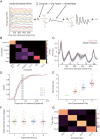
Experimental design. (A) Awake head-fixed mice viewed stimuli from a distance of 25 cm simultaneous with extracellular recoding via chronically implanted wire bundles. (B) Mice were randomly assigned to see Test stimuli on Day 1 (25%, naïve controls, green), Day 2 (33% of remaining mice, orange, 1 day of training), Day 3 (50% of remaining, blue, 2 days of training), or Day 4 (100% of remaining, magenta, 3 days of training). (C) The number of units recorded on each day was approximately uniform and evenly distributed between female and male mice (top and bottom of each bar). In total, we recorded 140 unique multi-unit channels from 56 mice. (D) Each training session consisted of 200 presentations of the sequence ABCD. Each element had a unique orientation and was held on screen for 150 ms and the full sequence lasted 600 ms. Sequences were separated from each other by a gray screen, held for a uniform random interval between 1 and 2 seconds. (E) During test sessions, mice were exposed to 600 presentations of randomly selected novel sequences: AxCD, ExCD, Ax→D, and Ex→D, where x indicates a random orientation (uniformly distributed ±60° around B) and → indicates an omitted third element (second element on screen for 300 ms, 50% of trials).

Fig. 2

MbTDR captures stimulus-dependent neural variability. (A) MbTDR, after Aoi and Pillow 2018) models PSTHs as a linear combination of covariates, unit factors, and shared basis functions. MbTDR discovers a low-rank representation, consisting of a small set of shared bases that are weighted differently for each unit (color code as in Fig. 1B). (B) Rank of optimal model, fit by maximum likelihood and a greedy rank estimation algorithm. Covariates were chosen to represent the experimental design and test stimulus (see the main text for details). Diagonal elements are the rank of each covariate, and off-diagonal elements represent the rank of interaction terms. (C) An example day-4-unit PSTH (binned at 25 ms with no smoothing, z-scored to zero spontaneous baseline firing and unit variance, as in all subsequent figures and analyses). The MbTDR prediction (black) matches the neural data (magenta, 95% confidence interval computed from observed Fisher information in gray). This unit had 4.41% held-out explained variance. (D) Empirical cumulative distribution functions (eCDFs) of explained variance across the 140 units. Each line represents the eCDF computed using held-out data from one test day (60 trials/day). The vertical black line is an estimate of explainable variance with a bootstrap 95% confidence interval. (E) Test days can be accurately decoded (each dot represents a single held-out pseudo-trial, x-axis jitter added for visibility). Due to our experiment and model design, Day 1 trials are automatically known. (D) Decoding error for x, the randomized angle of the second element, on the same held-out data (each dot is one pseudo-trial). The standard deviation on the error is 38.7°. (G) Confusion matrix for decoding the four primary stimulus types. The overall accuracy was 82.5%, whereas the chance for 60 trials is 25 +/− 2.7% (mean +/− SEM, gray box on the color bar shows 95% confidence interval of this estimate). The identity matrix would constitute perfect accuracy.

Fig. 3

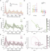
MbTDR reveals coordinated training-dependent change in neural activity. (A) Example PSTHs to AxCD (computed from the raw data, not the model fit). Units from trained mice (Days 2, 3, 4) that were strongly modulated by the day covariate (inset) are overlaid above example PSTHs from Day 1 units (green). Note the dip in firing after the onset of A in trained units. Some trained units drop as low as −0.5 on this z-scale, whereas no unit from Day 1 (the naïve group) drops below −0.15 in that same window. Early/late designations indicate the time windows used in (B). (B) Comparison of mean normalized firing rate across test days (again computed from the raw data, not model fit). Left shows mean firing rate in an early window (51–100 ms after onset of A), right during a late window (101–150 ms). There was no significant difference between trained and naïve groups in the early window (two-sided permutation test for difference in mean from Day 1, with a threshold set to P < 0.05/6 = 0.0083 for multiple comparisons: Day 2 P = 0.441; Day 3 P = 0.437; Day 4 P = 0.668). However, evoked firing in the late window was significantly lower in all trained groups (Day 2 P = 6.92e-4; Day 3 P = 0.0052; Day 4 P = 5.02e-4). The black dotted line marks the spontaneous baseline firing rate. (C) The first, second, and third principal components of evoked neural activity to ABCD in naïve mice, computed from the MbTDR fit (see Methods) with 95% confidence intervals. (F) Dynamic latent trajectory representation of the data in (C) in principle component space. Data were projected from 25-ms bins as in (D) to 1-ms bins using a Gaussian radial basis with 12.5-ms standard deviation. (E) Same as (C), but for the set of Day 4 units. The first component remains unchanged across days, whereas the second and third differ dramatically from Day 1. Note the dip in the second component from Day 4 around 100 ms, which mirrors decreased firing in the late window observed in (B). (F) Same as (D), but for Day 4 units. The second and third dimensions show rotational dynamics that, along with the first component, create a spiraling latent trajectory.

Fig. 4

Unexpected omissions cause prediction errors. (A) Example PSTHs from a Day 1 naïve unit comparing A/ExCD (blue) and A/Ex  D (red) trials (mean with 95% confidence intervals). (B) Example PSTH from Day 3. Omission of element C (in red) drives increased and sustained firing in a late window after its expected onset. (C) Difference PSTHs for all recorded units (red minus blue from the previous example, marked by an arrow in B). The Inset shows shared basis functions from MbTDR fit for the covariate (red) and interaction term ) (black). (D) Comparison of difference PSTHs in early (left) and late (right) windows (marked in C) after expected onset of element C. The early window is 51–100 ms after expected time of C onset, whereas late is 101–150 ms. There was no significant difference between trained and naïve groups in the early window (two-sided permutation test for difference in mean from Day 1, with a threshold set to P < 0.05/6 = 0.0083 for multiple comparisons: Day 2 P = 0.061; Day 3 P = 0.091; Day 4 P = 0.194). In the late window, however, firing was significantly higher on Days 2 and 4 (Day 2 P = 0.0012; Day 3 P = 0.016; Day 4 P = 5.02e-4). (D–E) The first and second principal components of neural activity for the ABD condition, in naïve (green) and fully trained (magenta) mice with 95% confidence intervals.

Fig. 5

Unexpected substitutions cause prediction errors. (A) Example PSTHs from a Day 1 naïve unit comparing all trials starting with A (blue) and E (black) with 95% confidence intervals. (B) As in (A) but for a Day 4 unit. Presentation of the trained A drives a sustained decrease in firing during a late window after its onset that is not present following E. (C) Difference PSTHs from all recorded units (black minus blue, illustrated with arrow in B). Inset shows shared basis functions from MbTDR fit for the covariate (black) and interaction term (red). (D) Comparison of difference PSTHs in early (left, 51–100 ms) and late (right, 101–150 ms) windows after onset of the first sequence element (A or E). There was a significant difference between naïve and trained groups in the early window (two-sided permutation test for difference in mean from Day 1, with a threshold set to P < 0.05/6 = 0.0083 for multiple comparisons: Day 2 P = 0.0062; Day 3 P = 0.23; Day 4 P = 0.0071). In the late window, the firing rate difference was significantly greater only on Day 4 (Day 2 P = 0.029; Day 3 P = 0.34; Day 4 P = 4.0e-6). (e–f) The first and second principal component of neural activity for the ABCD (light shade) and EBCD (dark shade) conditions with 95% confidence intervals. Both the first and second components show a significant dip following A, but not E, in the same late window.

Fig. 6

Temporal information in the V1 neural code. (A) Top: example pseudo-trial used for instantaneous time decoding. Each row represents a unit (all from the same test day), whereas each column represents one 25-ms time bin. Bottom: posterior probability distribution over possible time bins, calculated for the bin indicated by the shaded box above. In this case, the posterior correctly classifies the time bin based on a maximum a posteriori (MAP) estimate (marked with the gray triangle). (B) Dynamic latent trajectory representation of ABCD from Day 3 to 4 units demonstrate spiraling dynamics (as in Fig. 3) that create unique locations in PC space for each time point. (C) Temporal decoding accuracy across 60 held-out pseudo-trials and 30 time bins/trial for real (left, ~ 35 units per day) and simulated (right, 250 units per day, see Methods) data. “Soft accuracy” allows the decoder to be off by one time bin in either direction. Accuracy improved significantly with training (two-sided permutation test for difference in accuracy from Day 1, threshold set to 0.05/3 = 0.0167 to control for multiple comparisons. Real data: Day 2 P = 0.26; Day 3 P = 0.0059; Day 4 P < 1e-6. Simulated data: Day 2 P = 0.802; Day 3 P = 3.25e-4; Day 4 P = 6.29e-4). (D) Time decoding confusion matrices for naïve (left) and trained (right) units for real (top) and simulated (bottom) data. (E) Decoding soft accuracy in each time bin for simulated data. Training increases accuracy primarily at the beginning and ending of the sequence, which might be explained by the slight increase in evoked firing rate across days of training. Decoding is most accurate around element transitions (0, 150, 300, 450, 600 ms).

References

1. Aoi MC, Pillow JW. Model-Based Targeted Dimensionality Reduction for neuronal population data. Neural Inf Process Syst. 2018:31:6690–6699. Retrieved from http://pillowlab.princeton.edu/jpillow/. - PMC - PubMed
1. Aoi MC, Mante V, Pillow JW. Prefrontal cortex exhibits multidimensional dynamic encoding during decision-making. Nat Neurosci. 2020:23:1410–1420. 10.1038/s41593-020-0696-5. - DOI - PMC - PubMed
1. Atick JJ, Redlich AN. Convergent algorithm for sensory receptive field development. Neural Comput. 1993:5(1):45–60. 10.1162/neco.1993.5.1.45. - DOI
1. Audette NJ, Zhou WX, La Chioma A, Schneider DM. Precise movement-based predictions in the mouse auditory cortex. Curr Biol. 2022:32(22):4925–4940.e6. 10.1016/J.CUB.2022.09.064. - DOI - PMC - PubMed
1. Barlow HB. Possible principles underlying the transformations of sensory messages. In Sens Commun. 1961:1:217–234. 10.7551/mitpress/9780262518420.003.0013. - DOI
Publication types