Measurements of ear-canal geometry from high-resolution CT scans of human adult ears

Abstract

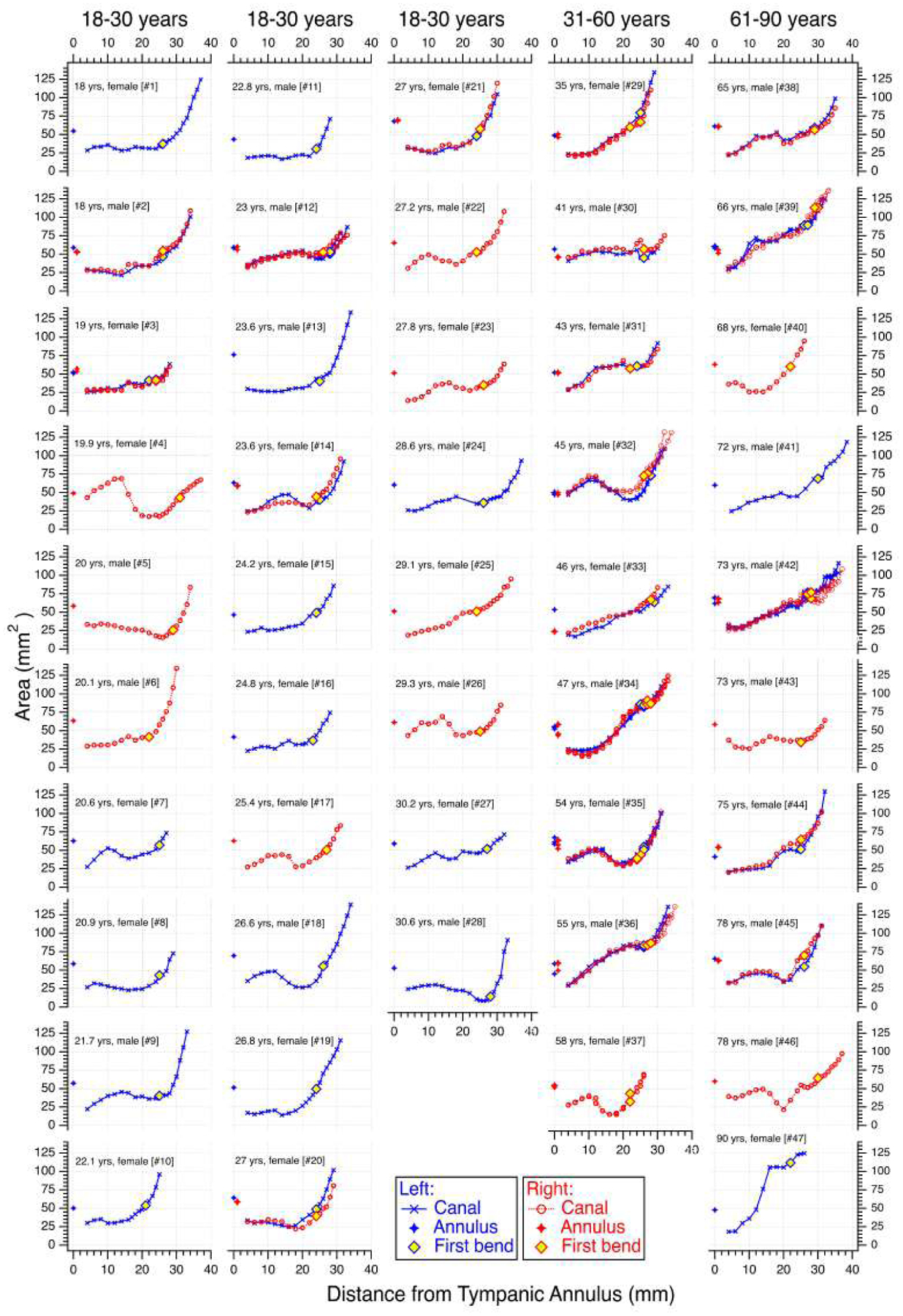
Description of the ear canal's geometry is essential for describing peripheral sound flow, yet physical measurements of the canal's geometry are lacking and recent measurements suggest that older-adult-canal areas are systematically larger than previously assumed. Methods to measure ear-canal geometry from multi-planar reconstructions of high-resolution CT images were developed and applied to 66 ears from 47 subjects, ages 18-90 years. The canal's termination, central axis, entrance, and first bend were identified based on objective definitions, and the canal's cross-sectional area was measured along its canal's central axis in 1-2 mm increments. In general, left and right ears from a given subject were far more similar than measurements across subjects, where areas varied by factors of 2-3 at many locations. The canal areas varied systematically with age cohort at the first-bend location, where canal-based measurement probes likely sit; young adults (18-30 years) had an average area of 44mm² whereas older adults (61-90 years) had a significantly larger average area of 69mm². Across all subjects ages 18-90, measured means ± standard deviations included: canals termination area at the tympanic annulus 56±8mm²; area at the canal's first bend 53±18mm²; area at the canal's entrance 97±24mm²; and canal length 31.4±3.1mm².

Keywords: Age related ear canal areas; CT Scan ear canal; Ear canal anatomy.

Figure 1:

CT scans: The original sagittal (orange, upper left), coronal (blue, upper right), and transverse (purple, lower left) planes upon opening the 3D Curved MPR tool. The yellow box indicates the right ear, as the transverse view is looking from inferior toward superior. Each pixel of the CT scan is assigned a gray scale number in Hounsfield units (HU). For the purposes of this work, air corresponds to −100 to −1024 HU, fat −30 to −100 HU, water 0 HU, muscle/soft tissue 20–100 HU, and bone 100–600 HU. Lower Right: Anatomical sagittal (orange), coronal (blue), and transverse (purple) planes with color coding that matches the OsiriX color schemes. The schematic is adapted from Egolf et al. (1993).

Figure 2:

Description of Step 1A. Upper: The original views in the sagittal (orange, upper left), coronal (blue, upper right), and transverse (purple, lower left) planes near the tympanic membrane (TM). Yellow circles indicate the tympanic annulus (TA) and the scutum (SC), which is a sharp bony projection along the TA to which the superior part of the tympanic membrane attaches. Lower: The MPR views after the sagittal (orange) axes were rotated in both the coronal and transverse views to align with the tympanic annulus and scutum, roughly parallel to the tympanic membrane. The MPR sagittal view shows the cross section at the tympanic annulus; the blue line in this sagittal view corresponds to the plane of the MPR coronal view to the right that is outlined in blue and the purple line corresponds to the MPR transverse view below that is outlined in purple. In the MPR transverse view, it is not possible to distinguish the anatomical landmarks (SC, TA) clearly from the 2D image. However, they can be seen within OsiriX by scrolling through adjacent sections and modifying the view slightly.

Figure 3:

Description of Steps 1B and 1C. Upper Panel: (Step 1B) The sagittal MPR plane at the canal’s termination defined in Fig. 2. The border between the bony tympanic annulus and the air is outlined in yellow, and the area is determined within the OsiriX software using the closed polygon tool. Lower Panel: (Step 1C) The center of the canal’s termination is defined within the sagittal plane; the wall-to-wall length along each of the coronal and transverse axes is measured within OsiriX (indicated by magenta distances), and the midpoint is half of the total (indicated by cyan distances); the center point is placed where the midpoints of these two axes intersect, and the center point is saved using the OsiriX spline tool as the most medial point of the canal’s central axis. This center point is shown in red in all three planes.

Figure 4:

Description of Steps 2A and 2B. Upper Panel: The spline mapping tool maps a curve in 3D space, and a straightened version of the curve is shown in the lower right box within the 3D curved MPR feature and indicates the distance between measurement points along the canal. The point at the canal’s termination is the point at the furthest left in this panel. In Step 2A, a point is placed with the spline mapping tool at the desired distance from the termination and at the estimated canals center while viewing the transverse and coronal views at the desired increment from the previous measurement. Here the “MPR Center Axis” box has been modified by adding additional information and larger writing than what is provided within OsiriX, to aid the reader. In Step 2B, the plane normal to the canal’s central axis is determined at each location, by adjusting the MPR sagittal plane angle within the transverse and coronal views so that the angles between the the surrounding canal wall and the sagittal plane are within 3° of each other within each of the transverse and coronal views. The resulting MPR sagittal plane defines the normal plane at the given canal location. Lower Panel: At each canal location, a normal plane (MPR sagittal plane, orange) is defined as perpendicular to the canals central axis. This plane is found by forcing the angles (cyan) between the surrounding canal walls (black) and the normal plane (orange) to be equal. The resulting normal plane has a 90° intersection with the central axis (red dotted line). The geometry is illustrated for multiple cases including when area along the canal length is constant, decreasing, increasing, and non-axially symmetric.

Figure 5:

Description of Step 2C. The MPR distance tool is used to determine the center point of the normal plane by finding the midpoint between the canal walls along the sagittal axes in both the MPR coronal and transverse planes. This example is shown at a distance of 6 mm from the termination, at point C along the MPR center axis. MPR Coronal View: Position the intersection of the sagittal and transverse axes at the midpoint along the sagittal axis by using the distance tool to determine the midpoint. First measure the wall-to-wall distance along the sagittal axis; here labelled “1” and shown as a dashed magenta line measured to be 9.53 mm. Next, draw a line from the canal wall along the sagittal axis that is half the distance; here labelled “2” and shown as a solid cyan line with length 4.76 mm. MPR Transverse View: Position the intersection of the sagittal and coronal axes at the midpoint along the sagittal axis by using the distance tool to determine the midpoint. First measure the wall-to-wall distance along the sagittal axis; here labelled “3” and shown as a dashed magenta line measured to be 6.35 mm. Next, draw a line from the canal wall along the sagittal axis that is half the distance; here labelled “4” and shown as a solid cyan line with length 3.17 mm. MPR Sagittal View: By design, the intersection of the coronal and transverse axes are centered in the sagittal view; their intersection defines the point for the central axis at this canal location.

Figure 6:

Description of Steps 2D and 2E . Left: (Step 2D) Step 2D is part of the interative process and includes (1) moving the initial spline point (open white circle) to the exact center point at the intersection of the axes from Step 2C (closed red circle); (2) confirming that the new location of the spline point is at its desired location along the canal; and (3) iterating Steps 2A-2D as needed. Right (Step 2E:) Measurement of the canal’s cross-sectional area (the same approach as Step 1B). The sagittal MPR plane at the canal’s location defines the plane normal to the canal’s central axis at the given location. The border between the canal wall and the air-filled canal is outlined in cyan, and the area is determined within the OsiriX software.

Figure 7:

Description of Step 3A, showing the definition of the entrance of the canal. Left: The MPR sagittal view (normal plane) includes canal wall around the entire perimeter, and an area can be measured. This location is the entrance to the canal because the MPR view 1 mm lateral includes the air space of the concha ear. Right: The MPR sagittal view (normal plane) 1 mm lateral to the view shown on the left. Here, the sagittal view includes an air connection to the concha (white arrow in sagittal view); this location is not part of the canal.

Figure 8:

Description of Steps 3B and 3C. Left: (Step 3B) The MPR transverse view shows the spline (red line) defining the central axis; the spline maps the curvature of the entire canal and may not always appear at the center of the canal due to the orientation and location of 2D images. The yellow star marks the first bend. Right: (Step 3C) The location of the canal’s first bend (yellow star) is at the most lateral sharp change in curvature of the canal’s central axis. This MPR sagittal plane is shown here at the location of the first bend, and this first-bend location is also indicated in the transverse view to the left.

Figure 9:

Canal areas, tympanic annulus areas, and first bend locations from three adult subjects (six ears) on which the method was developed. Measurements from three independent researchers, indicated with unique symbols, show relatively small variations. The area of the canal’s termination plane (defined by the tympanic annulus) is indicated at the distance of zero where it is defined. Measurements begin at 4 mm from the tympanic annulus and extend to the entrance of the canal, with one exception that the most lateral measurement for Subject #34 is not at the canal entrance because the CT scan was cut off medial to the entrance.

Figure 10:

All individual measurements made on 66 ears from 47 subjects. Columns indicate the three age cohorts. For better visualization, the area within the right tympanic annulus (distance 0) is shifted by 1 mm when it overlaps with the area within the left tympanic annulus. When multiple measurements exist on a given ear, they were always made by different researchers. Subject #18 has an entrance area of 159 mm² at a length of 35 mm, which is off the scale of the plot. The most lateral measurement for Subject #34 is not at the canal entrance because the CT scan was cut off medial to the entrance; the entrance was visible on the scans from all other subjects.

Figure 11:

Thin lines plot the mean canal area from each subject, calculated as the mean of all measurements from a given subject, including multiple investigators and multiple ears (Fig. 10). The population means ± their standard errors from the three age cohorts are also plotted; the population mean is plotted when there were at least 5 measurements at a given distance from the termination. Note, as the distance increases, some individual canals reach their termination at shorter distances leading to fewer points at the further distances; the younger group of ears has more individuals in it, likely leading to more canals being included at the longer lengths.

Figure 12:

Box plots that show the individual mean areas (upper row) and distances (lower row) for the indicated quantities categorized by age cohort; diamonds indicate individual points. Each box plot indicates the age cohortss median value with the red horizontal line, the upper and lower edges of each box define the 25th and 75th percentiles, and the notch height is the median ± 1.57 times the interquartile range divided by $\sqrt{\text{N}}$ where N is the number of data points; the notches can extend beyond the 25th or 75th percentiles when the sample size is small due to the division by $\sqrt{\text{N}}$.

Figure 13:

Comparisons of the range of area measurements from this work to the range from Stinson and Lawton (1989). The yellow diamonds indicate the average first bend locations and corresponding areas for each subject, and the black asterisks indicate the canal length and corresponding area for each subject. (*) Stinson and Lawton (1989) summarized 14 cadaver ears that were each scaled to fit to a length of 30 mm. (**) The range plotted from this work excluded the measurements from subject #47 (age 90) that was an extreme outlier. (***) One subject did not have an entrance measurement due to the CT scan being cut off.

References

1. Balouch A, 2021. Describing the geometry of the ear canal from CT scans. Undergraduate thesis, Smith College, Northampton, MA. URL https://scholarworks.smith.edu/theses/2316/
1. Bland JM, Altman DG, 1986. Statistical methods for assessing agreement between two methods of clinical measurement. The Lancet, 307–310. - PubMed
1. Egolf DP, Nelson DK, Howell HC, Larson VD, May 1993. Quantifying ear-canal geometry with multiple computer-assisted tomographic scans. J. Acoust. Soc. Am 93 (5), 2809–2819. - PubMed
1. Farmer-Fedor BL, Rabbitt RD, 2002. Acoustic intensity, impedance and reflection coefficient in the human ear canal. J. Acoust. Soc. Am 112, 600620. - PubMed
1. Feeney MP, 2013. Eriksholm workshop: Wideband absorbance measures of the middle ear. Ear Hear 34, Supplement 1. - PubMed
Publication types