Regional patterns of human cortex development correlate with underlying neurobiology

Abstract

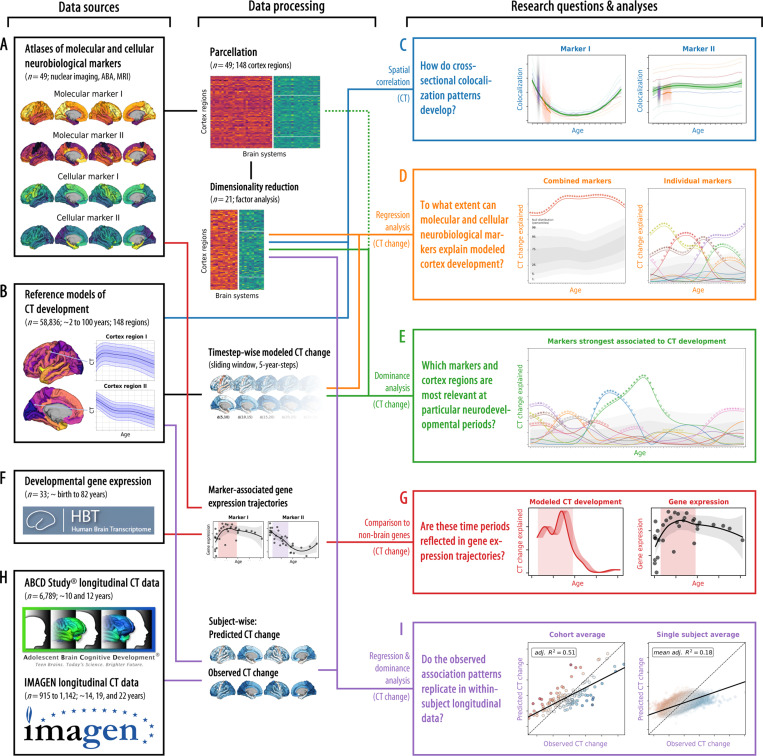
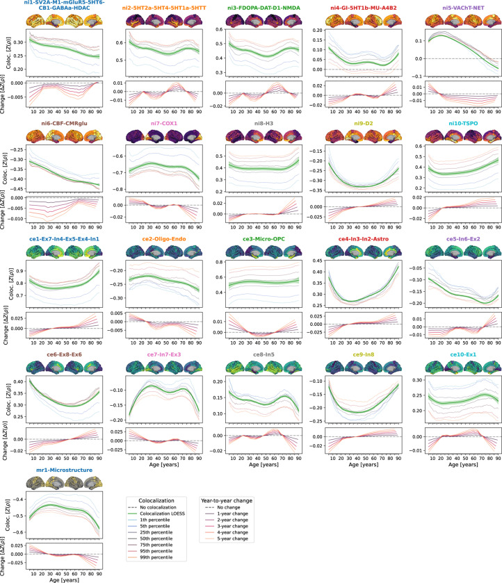
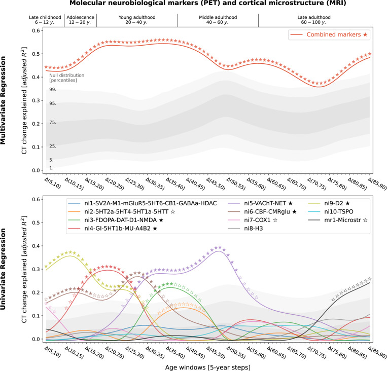
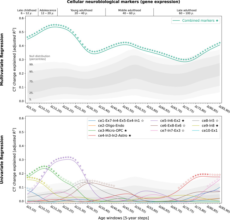
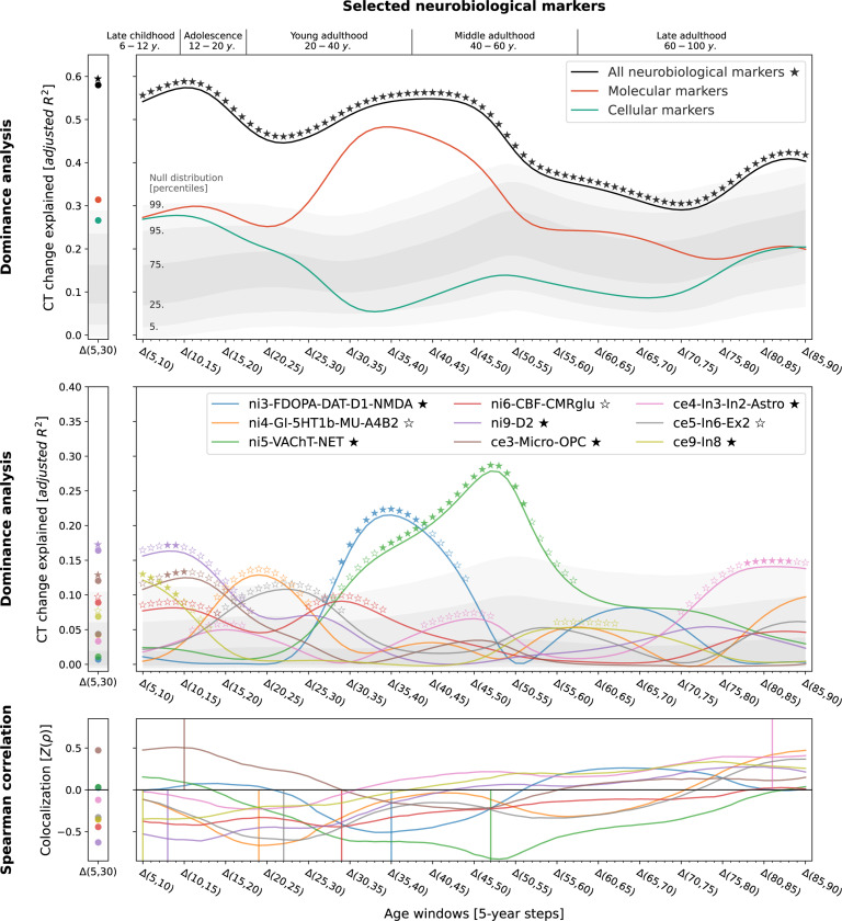
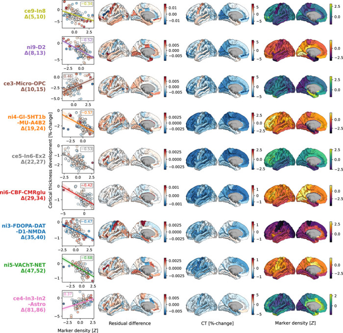
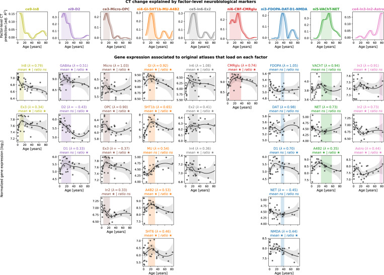
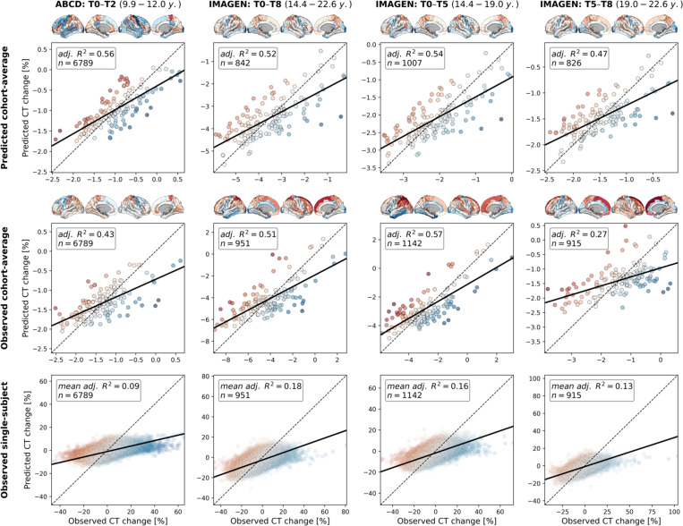
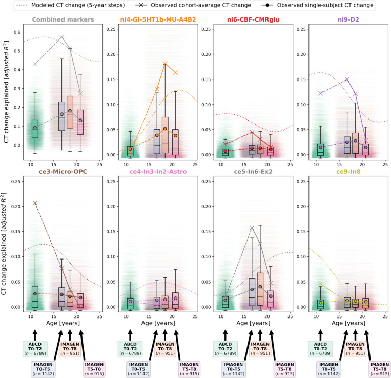
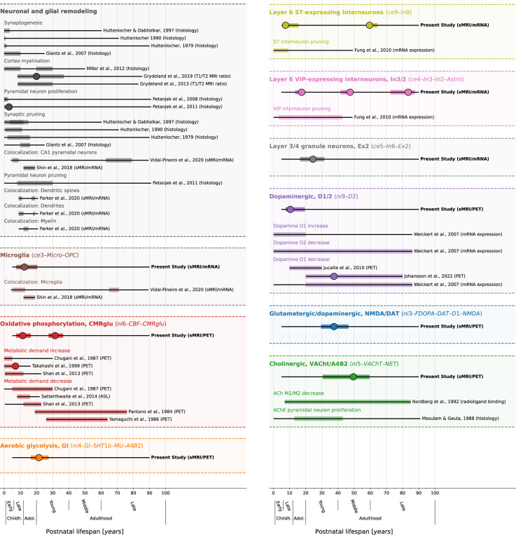
Human brain morphology undergoes complex changes over the lifespan. Despite recent progress in tracking brain development via normative models, current knowledge of underlying biological mechanisms is highly limited. We demonstrate that human cortical thickness development and aging trajectories unfold along patterns of molecular and cellular brain organization, traceable from population-level to individual developmental trajectories. During childhood and adolescence, cortex-wide spatial distributions of dopaminergic receptors, inhibitory neurons, glial cell populations, and brain-metabolic features explain up to 50% of variance associated with a lifespan model of regional cortical thickness trajectories. In contrast, modeled cortical thickness change patterns during adulthood are best explained by cholinergic and glutamatergic neurotransmitter receptor and transporter distributions. These relationships are supported by developmental gene expression trajectories and translate to individual longitudinal data from over 8,000 adolescents, explaining up to 59% of developmental change at cohort- and 18% at single-subject level. Integrating neurobiological brain atlases with normative modeling and population neuroimaging provides a biologically meaningful path to understand brain development and aging in living humans.

Keywords: Cortex; Cortical thickness; Dominance analysis; Longitudinal; Neurodevelopment; Neuronal cell types; Neurotransmitters; Normative modeling; Nuclear imaging.

Fig. 1:. Study overview

The workflow of the present study, from data sources (left side) to data processing and analysis method (middle) to the research questions and results (right side). (A) A collection of postmortem “cellular” and in vivo “molecular” brain atlases was parcellated and dimensionality reduced. (B) “Modeled” predicted CT data was extracted from a normative model. (C) We calculated the colocalization between neurobiological markers and CT at each point throughout the lifespan (see Fig. 2). (D) We evaluated how combined and individual neurobiological markers could explain lifespan CT change (see Figs. 3 and 4). (E) The strongest associated markers were examined in detail, accounting for shared spatial patterns (see Fig. 5). (F) A developmental gene expression dataset was used to generate trajectories of gene expression associated with each neurobiological marker. (G) Periods in which CT change was significantly explained were validated in developmental gene expression data (see Fig. 7). (H) Single-subject longitudinal data was extracted from two developmental cohorts. (I) Findings based on the normative model were validated in single-subject data (see Fig. 8). Abbreviations: CT cortical thickness, ABA = Allen Brain Atlas, MRI = magnetic resonance imaging. Here, data plots are employed for demonstration purposes; for definitions of plot elements, please refer to the individual figures as refererred to above, similarly, source data are provided in Source Data files of each following figure. ABCD Study^®, Teen Brains. Today’s Science. Brighter Future.^® and the ABCD Study Logos are registered marks of the U.S. Department of Health & Human Services (HHS).

Fig. 2:. Colocalization between cross-sectional modeled CT and neurobiologial markers across the lifespan

Lifespan trajectories of colocalization between neurobiological markers and modeled cross-sectional CT. For each marker, the upper panel shows a surface projection of the parcellated data; yellow-violet: nuclear imaging markers, yellow-green: gene-expression, yellow-gray: microstructural; yellow = higher density. The center panel shows the marker’s colocalization trajectory: Z-transformed Spearman correlation coefficients are shown on the y axis, age on the x axis; blue-to-orange lines indicate percentiles of modeled CT data (see legend, note that these do not show actual percentiles of colocalization strengths); the green line (LOESS = locally estimated scatterplot smoothing) was smoothed through the percentile data to highlight trajectories (shades: 95% confidence intervals). The lower panel shows year-to-year changes (y axis) derived from the LOESS line in the upper plot. See Fig. S7 for trajectories including ABCD and IMAGEN subjects and Fig. S8 for trajectories split by sex. Abbreviations: Coloc. = colocalization, SV2A = synaptic vesicle glycoprotein 2A, M1 = muscarinic receptor 1, mGluR5 = metabotropic glutamate receptor 5, 5HT1a/1b/2a/4/6 = serotonin receptor 1a/2a/4/6, CB = cannabinoid receptor 1, GABAa = γ-aminobutyric acid receptor A, HDAC = histone deacetylase, 5HTT = serotonin transporter, FDOPA = fluorodopa, DAT = dopamine transporter, D1/2 = dopamine receptor 1/2, NMDA = N-methyl-D-aspartate glutamate receptor, GI = glycolytic index, MU = mu opioid receptor, A4B2 = α4β2 nicotinic receptor, VAChT = vesicular acetylcholine transporter, NET = noradrenaline transporter, CBF = cerebral blood flow, CMRglu = cerebral metabolic rate of glucose, COX1 = cyclooxygenase 1, H3 = histamine receptor 3, TSPO = translocator protein, Microstr = cortical microstructure, Ex = excitatory neurons, In = inhibitory neurons, Oligo = oligodendrocytes, Endo = endothelial cells, Micro = microglia, OPC = oligodendrocyte progenitor cells, Astro = astrocytes. Source data are provided as a Source Data file.

Fig. 3:. Modeled lifespan CT change patterns explained by molecular neurobiological markers and cortical microstructure

Associations between modeled lifespan CT change and neurobiological markers derived from imaging modalities. Developmental periods covered by this study as defined by Kang et al. are shown on top. Time periods were aligned to the center of each modeled CT change step (e.g., Δ(5,10) = 7.5). Colored lines show the amount of spatial modeled CT change variance explained (y axis) by the combined markers (upper) or each marker individually (lower) throughout the lifespan (x axis). Each y value represents the results of one multiple (upper) or single (lower) linear regression model predicting CT change across regions from neurobiological marker densities across regions. Stars indicate positive-sided significance of each regression model based on null regression models estimated on permuted marker maps; ★: FDR-corrected across all tests shown in each panel of the plot; ☆: nominal p < 0.05. To provide an estimate of the actual observed effect size, gray areas show the distributions of modeled CT change explained by permuted marker maps (n = 10,000). For the lower panel, null results were combined across marker maps. See Fig. S6C for all CT change maps, and Fig. S4 for all predictor maps. Abbreviations: CT = cortical thickness, PET = positron emission tomography, MRI = magnetic resonance imaging, FDR = false discovery rate, see Fig. 2 for abbreviations used in neurobiological marker names. Source data inlcuding exact p values are provided as a Source Data file.

Fig. 4:. Modeled lifespan CT change patterns explained by cellular neurobiological markers

Associations between modeled lifespan CT change and neurobiological markers derived from mRNA expression data. The figure layout and shown plot elements correspond to Fig. 4. See Fig. S6C for all CT change maps, and Fig. S4 for all predictor maps. Abbreviations: CT = cortical thickness, see Fig. 2 for abbreviations used in neurobiological marker names. Source data inlcuding exact p values are provided as a Source Data file.

Fig. 5:. In-depth analysis of the neurobiological markers most relevant for explaining modeled CT change patterns across the lifespan

Modeled lifespan CT change explained by neurobiological markers, selected from the univariate analyses (Figs. 3 and 4; 9 FDR-corrected significant markers). See Fig. 3 for descriptions of global plot elements. Top: overall explained modeled CT change variance, the two colored lines highlight contributions of molecular and cellular markers. Middle: Marker-wise contributions to the overall explained spatial variance. Note that, as the used total dominance statistic describes the average R² associated with each predictor relative to the “full model” R², the sum of the predictor-wise values at each timepoint in the middle plot equals the R² values expressed in the upper panel. Bottom: Spearman correlations between modeled CT change and markers to visualize the sign of the association patterns. Abbreviations: CT = cortical thickness, see Fig. 2 for abbreviations used in neurobiological marker names. Source data including exact p values are provided as a Source Data file.

Fig. 6:. Cortex-regional influences on modeled CT change patterns explained by most relevant neurobiological markers

Regional influences on explained modeled CT change. Each row shows one of the 9 markers included in dominance analyses. Scatterplots: Correlation between modeled CT change at the respective predictor’s peak timestep (y axis) and the predictor map, corresponding to panel A-bottom. The first surface shows the residual difference maps calculated for each marker, highlighting the most influential regions on modeled CT change association effects. For illustration purposes, the second and third surface show modeled CT change and the spatial distribution associated with the marker. Colorbars map (i) residual difference, (ii) percent-change, and (iii) z-transformed marker density; individual colorbars were not labelled to maintain readability. See Fig. S14 for all residual difference maps, Fig. S6C for all modeled CT change maps, and Fig. S4 for all predictor maps. Abbreviations: CT = cortical thickness, see Fig. 2 for abbreviations used in neurobiological marker names. Source data are provided as a Source Data file.

Fig. 7:. Validation of CT model-based results in developmental gene expression data

First row: Modeled CT change explained by individual neurobiological markers, exactly corresponding to univariate results in Figs. 3 and 4. X values are aligned to the first year of each tested modeled CT change time period (e.g., Δ(5,10) is aligned to 5 years on x-axis). Shades following each line visualize other possible alignments (Δ(5,10) is aligned to 6, 7, 8, 9, or 10 years). Vertical shaded boxes indicate time periods in which CT change was explained significantly (FDR). Following rows: Normalized log₂-transformed gene expression trajectories for maxiumally 5 original atlases that loaded on factor-level neurobiological markers with λ > |0.3| (c.f., Fig. S15). Gene expression for each marker was derived from related single genes or from averaging across gene sets. Grey dots indicate average neocortical expression of individual subjects. Black lines and shades show locally estimated scatterplot smoothing (LOESS) curves with 95% confidence intervals. Associations were tested for by averaging the LOESS data within and outside of each respective time period and comparing mean and ratio against null data randomly sampled from non-brain genes (positive-sided exact p values). ★: FDR-corrected across all tests; ☆: nominal p < 0.05. Abbreviations: CT = CT change, adj. = adjusted, FDR = false discovery rate, ns = not significant, see Fig. 2 for abbreviations used in neurobiological marker names. Source data inlcuding exact p values are provided as a Source Data file.

Fig. 8:. Validation of overall explain CT change in ABCD and IMAGEN datasets

Explained spatial CT change variance in ABCD and IMAGEN data. The overall model performance is illustrated as scatter plots contrasting predicted CT change (y axis) with observed CT change (x axis). Scatters: single brain regions, color-coded by prediction error. Continuous line: linear regression fit through the observations. Dashed line: theoretical optimal fit. Brains: prediction errors corresponding to scatters. Rows: upper: cohort-average predicted by the reference (Braincharts) model, lower sample size due to subjects dropped during model adaptation (see Methods); middle: observed cohort-average (ComBat-harmonized); lower: observed single-subject values (ComBat-harmonized), one regression model was calculated for each subject, but the results were combined for illustration purposes. Abbreviations: CT = cortical thickness, adj. = adjusted. Group-level source data are provided as a Source Data file.

Fig. 9:. Validation of individual marker-level results in ABCD and IMAGEN datasets

Explained spatial CT change variance with a focus on the individual neurobiological markers. Subplots for the combined analysis and each individual marker show: modeled CT change as presented in Figs. 3 and 4 (dotted line); observed cohort-average CT change (cross markers); and observed single-subject CT change (boxplots and dot markers). For each subject, one horizontal line at their individual R² value ranges from their age at beginning and end of each time span. Boxplots show the distribution of individual values for each time span (boxes: lower-bound: 25^th, center: 50^th, upper-bound: 75^th percentile; whiskers: 1.5 × interquartile range). Note that the first subplot (Combined markers) corresponds to the data presented in Fig. 8. See Figs. S22 and S23 for detailed results. Abbreviations: CT = cortical thickness, see Fig. 2 for abbreviations used in neurobiological marker names. Group-level source data are provided as a Source Data file.

Fig. 10:. Summary of study findings in the context of prior literature on humans

Condensed visualization of the reported results (first line of each block, emphasized are neurobiological markers that showed consistent results) in context with related results of previous human studies investigating similar biological processes or cell populations (lines below)^{–,–,,,,–,–,,–}. We do not claim this collection to be exhaustive. In the left upper panel, we show studies investigating general cellular remodeling processes; in the other panels, each header indicates one neurobiological marker with associated studies below. Each thin black line overlaid by a colored bar indicates results from one study. If a study reported multiple results pertaining to the same process (e.g., from two different brain regions), bars were laid over each other (Data S5 for individual listings). Thin black lines: overall time span investigated. Colored overlay: time period in which the respective study target was reported to show developmental changes (present study: nominal p < 0.05), independent of the sign of the association. Large dots: Timepoint of the maximum association. See also Fig. S28 and Data S5 for a more comprehensive overview including various topics. Abbreviations: ST = somatostatin, CR = calretinin, sMRI = structural MRI, CBF = cerebral blood flow, PET = positron emission tomography, ASL = arterial spin labeling, ACh(E) = acetylcholine (esterase), see Fig. 2 for abbreviations used in neurobiological marker names. Source data are provided as a Source Data file.

References

1. Bethlehem R. A. I. et al. Brain charts for the human lifespan. Nature 604, 525–533 (2022). - PMC - PubMed
1. Gogtay N. et al. Dynamic mapping of human cortical development during childhood through early adulthood. Proceedings of the National Academy of Sciences 101, 8174–8179 (2004). - PMC - PubMed
1. Rutherford S. et al. Charting brain growth and aging at high spatial precision. eLife 11, e72904 (2022). - PMC - PubMed
1. Vanderhaeghen P. & Polleux F. Developmental mechanisms underlying the evolution of human cortical circuits. Nat Rev Neurosci 24, 213–232 (2023). - PMC - PubMed
1. Erus G. et al. Imaging Patterns of Brain Development and their Relationship to Cognition. Cerebral Cortex 25, 1676–1684 (2015). - PMC - PubMed
Publication types