. 2023 May 19;9(20):eadd0560.
doi: 10.1126/sciadv.add0560. Epub 2023 May 19.

Convergent genomic signatures of local adaptation across a continental-scale environmental gradient

Affiliations

Convergent genomic signatures of local adaptation across a continental-scale environmental gradient

Lucas R Moreira et al. Sci Adv. .

Abstract

Convergent local adaptation offers a glimpse into the role of constraint and stochasticity in adaptive evolution, in particular the extent to which similar genetic mechanisms drive adaptation to common selective forces. Here, we investigated the genomics of local adaptation in two nonsister woodpeckers that are codistributed across an entire continent and exhibit remarkably convergent patterns of geographic variation. We sequenced the genomes of 140 individuals of Downy (Dryobates pubescens) and Hairy (Dryobates villosus) woodpeckers and used a suite of genomic approaches to identify loci under selection. We showed evidence that convergent genes have been targeted by selection in response to shared environmental pressures, such as temperature and precipitation. Among candidates, we found multiple genes putatively linked to key phenotypic adaptations to climate, including differences in body size (e.g., IGFPB) and plumage (e.g., MREG). These results are consistent with genetic constraints limiting the pathways of adaptation to broad climatic gradients, even after genetic backgrounds diverge.


Figures

Fig. 1.
Fig. 1.. Environmental variation across the ranges of Downy and Hairy Woodpeckers.
(A) Map depicting the sympatric range of Downy and Hairy Woodpeckers, the location of the study samples (dots), and their respective populations of origin (large circles). Each population has a sample size of n = 10. Colors on the map are based on the principal components analysis (PCA) of the bioclimatic data shown in (B). We converted scores of the first three principal components (PCs) into values of RGB (PC1: red; PC2: green; PC3: blue) to represent variation in climate. Thus, similar colors represent similar climates. (B) PCA of the 19 bioclimatic variables from the WorldClim database (36). Background points (gray) represent 1000 randomly sampled points across the sympatric range of both focal species. Points from each population are represented by different colors. (C) Biplot of the PCA of bioclimatic data indicating the correlations among variables and the direction and magnitude of their contribution to the first two PCs of the PCA. AK, Alaska; MW, Midwest; NE, Northeast; NR, Northern Rockies; NW, Pacific Northwest; SE, Southeast; SR: Southern Rockies.
Fig. 2.
Fig. 2.. GEA analysis and genomic convergence in Downy and Hairy Woodpeckers.
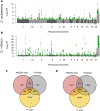
Manhattan plots showing candidate genes associated with the first PC (PC1) of (A) temperature and (B) precipitation in Downy Woodpecker and (C) temperature and (D) precipitation in Hairy Woodpecker. Each dot represents the median LRT statistic estimated for a given 50-SNP sliding window along the genome. Colors differentiate consecutive pseudochromosomes. Venn diagram describing the total number of candidate genes from the ANGSD-asso latent model associated with (E) temperature and (F) precipitation shared by Downy (left) and Hairy (right) Woodpeckers. Density plot shows the cumulative hypergeometric distributions of the probability of observing a given number of overlapping candidate genes. The red dashed line indicates the empirical observation.
Fig. 3.
Fig. 3.. Population-structure outliers and method intersection.
Manhattan plots showing outliers windows of population structure according to PCAdapt in Downy (A) and Hairy (B) Woodpeckers. Each dot represents the median −log10(P) estimated for a given 50-SNP sliding window along the genome. Gray colors differentiate consecutive pseudochromosomes. Green dots indicate candidate loci. Venn diagrams describing the intersection of candidate windows between ANGSD-asso, PCAdapt, and H-scan in Downy (C) and Hairy (D) Woodpeckers.
Fig. 4.
Fig. 4.. Correlates of the number of FST-outlier windows in Downy and Hairy Woodpeckers.
Heatmaps of FST-outlier windows and correlates across population comparisons in Downy (left) and Hairy (right) Woodpeckers. Shown are heatmaps of the number of genomic windows detected in the FST-outlier analysis for each population comparison (A and B), the genome-wide FST across all population comparisons (C and D), and the average environmental dissimilarity among populations (E and F) calculated as the Euclidean distance between PCs of the 19 bioclimatic variables from the WorldClim database (36). AK, Alaska; MW, Midwest; NE, Northeast; SE, Southeast; NW, Pacific Northwest; NR, Northern Rockies; SR, Southern Rockies.
Fig. 5.
Fig. 5.. IGFBP genes show convergent signatures of selection in Downy and Hairy Woodpeckers.
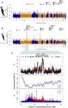
Manhattan plot comparing Alaska (AK) and the Southeast (SE) population in (A) Downy and (B) Hairy Woodpeckers. Each dot represents the FST value estimated for a given 50-kb sliding window along the genome. Colors differentiate consecutive pseudochromosomes. The red line indicates the genome-wide mean FST (Downy FST = 0.12; Hairy FST = 0.13), and the blue line indicates the cutoff value of 5 SDs above the mean for a window to be considered an outlier (Downy FST = 0.32; Hairy FST = 0.34). Squares indicate the location of key annotated genes found within outlier windows. (C) Genomic signatures of selective sweep in the comparison between AK and the SE in a segment of pseudochromosome 2 of Downy Woodpecker. Top: FST between AK and the SE across 10-kb windows in 2-kb increments. The red line represents the local polynomial regression fit, and the blue rectangles indicate the location of genes. Five key genes with elevated FST are indicated by different colors. Middle: Nucleotide diversity in AK (black line) and the SE (blue line). Bottom: Average length of pairwise homozygosity tracts for each SNP (H) along this segment of pseudochromosome 2 in the AK (red) and Eastern (blue) population. E, East (NE + SE + MW).
Fig. 6.
Fig. 6.. A candidate gene for plumage variation in Hairy Woodpecker.
(A) Manhattan plot showing FST values between Pacific Northwest (NW) and NR estimated for 50-kb sliding windows along the genome with 10-kb increments. Colors differentiate consecutive pseudochromosomes. The red line indicates the genome-wide mean FST (FST = 0.05), and the blue line indicates the cutoff value of 5 SDs above the mean for a window to be considered outlier (FST = 0.11). (B) Average length of pairwise homozygosity tracts for each SNP (H) for the NW (dark individuals) and NR (white individuals) population in a segment of pseudochromosome 7 containing the gene melanoregulin (MREG). (C) Genotypes for each SNP located in the segment containing the MREG gene separated by population. Blue, homozygous for the reference allele; pink, heterozygous; red, homozygous for the alternative allele; brown, missing genotype. AK, Alaska; MW, Midwest; NE, Northeast; SE, Southeast; SR, Southern Rockies; NR, Northern Rockies; NW, Northwest.

Comment in

Similar articles

Cited by

References

    1. A. E. Lobkovsky, E. V. Koonin, Replaying the tape of life: Quantification of the predictability of evolution. Front. Genet. 3, 246 (2012). - PMC - PubMed
    1. V. Orgogozo, B. Morizot, A. Martin, The differential view of genotype-phenotype relationships. Front. Genet. 6, 179 (2015). - PMC - PubMed
    1. E. B. Rosenblum, C. E. Parent, E. E. Brandt, The molecular basis of phenotypic convergence. Annu. Rev. Ecol. Evol. Syst. 45, 203–226 (2014).
    1. D. L. Stern, V. Orgogozo, The loci of evolution: How predictable is genetic evolution? Evolution 62, 2155–2177 (2008). - PMC - PubMed
    1. G. L. Conte, M. E. Arnegard, C. L. Peichel, D. Schluter, The probability of genetic parallelism and convergence in natural populations. Proc. R. Soc. B 279, 5039–5047 (2012). - PMC - PubMed