Bayesian Data Selection

Abstract

Insights into complex, high-dimensional data can be obtained by discovering features of the data that match or do not match a model of interest. To formalize this task, we introduce the "data selection" problem: finding a lower-dimensional statistic-such as a subset of variables-that is well fit by a given parametric model of interest. A fully Bayesian approach to data selection would be to parametrically model the value of the statistic, nonparametrically model the remaining "background" components of the data, and perform standard Bayesian model selection for the choice of statistic. However, fitting a nonparametric model to high-dimensional data tends to be highly inefficient, statistically and computationally. We propose a novel score for performing data selection, the "Stein volume criterion (SVC)", that does not require fitting a nonparametric model. The SVC takes the form of a generalized marginal likelihood with a kernelized Stein discrepancy in place of the Kullback-Leibler divergence. We prove that the SVC is consistent for data selection, and establish consistency and asymptotic normality of the corresponding generalized posterior on parameters. We apply the SVC to the analysis of single-cell RNA sequencing data sets using probabilistic principal components analysis and a spin glass model of gene regulation.

Keywords: Bayesian nonparametrics; Bayesian theory; Stein discrepancy; consistency; misspecification.

Figure 10:

Behavior of the Stein volume criterion $𝒦$, the foreground marginal likelihood with a background volume correction ${𝒦}^{\left(\text{a}\right)}$, and the foreground marginal nksd ${𝒦}^{\left(\text{b}\right)}$ on toy examples. The plots show the results for 5 randomly generated data sets (thin lines) and the average over 100 random data sets (bold lines). Here, unlike Figure 2, the Pitman-Yor expression for $m_{ℬ}$ is used (Equation 3), with $\alpha =0.5,\nu =1$, and $D=0.2$.

Figure 11:

Estimated $T$ for increasing number of data samples, for 10 independent parameter samples from the prior. The median value at $N=2000$ is $\hat{T}=0.052$.

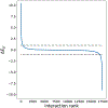
Figure 12:

Posterior mean interaction energies $\mathrm{\Delta }{E}_{j{j}^{\mathrm{\prime }}}$ for all selected genes, sorted. Dotted lines show the thresholds for strong interactions (set by visual inspection).

Figure 13:

Posterior mean interaction energies $\mathrm{\Delta }{E}_{j{j}^{\mathrm{\prime }}}$ for the glass model applied to all 200 genes in the MALT data set (rather than the selected 187). Genes shown are the same as in Figure 8, for visual comparison.

Figure 14:

Comparison of the 187 selected genes and 13 excluded genes using data selection. (a) Violin plot of ${\bar{\sigma }}_j$ over all excluded and selected genes $j$, respectively, when applying the model to all 200 genes, where ${\bar{\sigma }}_j$ is the mean posterior standard deviation of the interaction energies $\mathrm{\Delta }{E}_{j{j}^{\mathrm{\prime }}}$ for gene $j$, that is, ${\bar{\sigma }}_j≔\frac{1}{d-1}{\sum }_{j^{\mathrm{\prime }}\ne j} \text{std}\left(\mathrm{\Delta }{E}_{j{j}^{\mathrm{\prime }}}\mid \right.$ data $)$. (b) Violin plot of $f_j$ over all excluded and selected genes $j$, respectively, where $f_j$ is the fraction of cells with count equal to zero for gene $j$. The data selection procedure excluded all genes with more than $85\mathrm{\%}$ zeros and selected all genes with fewer than $85\mathrm{\%}$ zeros.

Figure 1:

A simple example illustrating the data selection problem.

Figure 2:

Behavior of the Stein volume criterion $𝒦$, the foreground marginal likelihood with a background volume correction ${𝒦}^{\left(a\right)}$, and the foreground marginal NKSD ${𝒦}^{\left(\text{b}\right)}$ on toy examples. Here, we set $m_{ℬ}=5r_{ℬ}$. The plots show the results for 5 randomly generated data sets (thin lines) and the average over 100 random data sets (bold lines).

Figure 3:

Data selection in the probabilistic PCA model.

Figure 4:

(a,b) Histograms of gene expression (after pre-processing), i.e., $X_j^{\left(1\right)},\dots ,X_j^{\left(N\right)}$, for genes $j$ selected to be included in the foreground space based on the log SVC ratio $\text{log}{𝒦}_j-\text{log}{𝒦}_0$. The estimated density under the pPCA model is shown in blue. (c,d) Histograms of example genes selected to be excluded. Higher ranks (in each title) correspond to larger log SVC ratios.

Figure 5:

Scatterplot comparison and projected marginals of the leave-one-out log SVC ratio, $\text{log}{𝒦}_j-\text{log}{𝒦}_0$ (with $m_{{ℬ}_j}=m_{{ℱ}_0}-m_{{ℱ}_j}$), and the conventional full model criticism score, $\text{log}{ℰ}_j-\text{log}{ℰ}_0$, for each gene.

Figure 6:

(a) Comparison of the conventional criticism score, for each gene $j$, and the fraction of cells that show zero expression of that gene $j$ in the raw data. Spearman $\rho =0.89,p<0.01$. (b) Same as (a) but with the log SVC ratio. Spearman $\rho =0.98,p<0.01$. In orange are genes that would be included when using a background model with $c_{ℬ}=20$ and in blue are genes that would be excluded. (c) Same as (a) for a data set taken from a MALT lymphoma (Section D.5). Spearman $\rho =0.81,p<0.01$. (d) Same as (b) for the MALT lymphoma data set. Spearman $\rho =0.99,p<0.01$.

Figure 7:

(a) Histogram of log SVC ratios $\text{log}{𝒦}_j-\text{log}{𝒦}_0$ for all 200 genes in the data set (with $m_{{ℬ}_j}=m_{{ℱ}_0}-m_{{ℱ}_j}$). Dotted lines show the value of the volume correction term in the SVC for different choices of background model complexity $c_{ℬ}$; for each choice, genes with $\text{log}{𝒦}_j-\text{log}{𝒦}_0$ values above the dotted line would be excluded from the foreground subspace based on the SVC. (b) Posterior mean of the first two latent variables $\left(z_1\right.$ and $\left.z_2\right)$, with the pPCA model applied to the genes selected with a background model complexity of $c_{ℬ}=10$ (keeping 23 genes in the foreground). (c-e) Same as (b), but with $c_{ℬ}=20$ (keeping 38 genes), $c_{ℬ}=40$ (keeping 87 genes) and $c_{ℬ}=60$ (keeping all 200 genes). In (a)-(d), the points are colored using the $z_1$ value when $c_{ℬ}=60$.

Figure 8:

Posterior mean interaction energies $\mathrm{\Delta }{E}_{j{j}^{\mathrm{\prime }}}≔J_{j{j}^{\mathrm{\prime }}21}+J_{j{j}^{\mathrm{\prime }}12}-J_{j{j}^{\mathrm{\prime }}22}-J_{j{j}^{\mathrm{\prime }}11}$ for a subset of the selected genes. For visualization purposes, weak interactions $\left(\left|\mathrm{\Delta }{E}_{j{j}^{\mathrm{\prime }}}\right|\le 1\right)$ are set to zero, and genes with less than 10 total strong connections are not shown. Genes are sorted based on their (signed) projection onto the top principal component of the $\mathrm{\Delta }E$ matrix.

Figure 9:

Comparison of posterior mean interaction energies $\mathrm{\Delta }{E}_{j{j}^{\mathrm{\prime }}}$ for a model applied to all 200 genes (pre-data selection) to those learned from a model applied to the selected foreground subspace (post-data selection). Each point corresponds to a pairwise interaction between two of the selected 187 genes.

References

1. Alon Uri. An Introduction to Systems Biology: Design Principles of Biological Circuits. CRC Press, July 2019.
1. Anastasiou Andreas, Barp Alessandro, Briol François-Xavier, Ebner Bruno, Gaunt Robert E, Ghaderinezhad Fatemeh, Gorham Jackson, Gretton Arthur, Ley Christophe, Liu Qiang, Mackey Lester, Oates Chris J, Reinert Gesine, and Swan Yvik. Stein's method meets statistics: A review of some recent developments. arXiv preprint arXiv:2105.03481, May 2021.
1. Banerjee Onureena, Ghaoui Laurent El, and d'Aspremont Alexandre. Model selection through sparse maximum likelihood estimation for multivariate Gaussian or binary data. Journal of Machine Learning Research, 9(Mar):485–516, 2008.
1. Barp Alessandro, Briol Francois-Xavier, Duncan Andrew B, Girolami Mark, and Mackey Lester. Minimum Stein discrepancy estimators. arXiv preprint arXiv:1906.08283, June 2019.
1. Barron Andrew R. Uniformly powerful goodness of fit tests. The Annals of Statistics, 17 (1):107–124, 1989.
LinkOut - more resources