The stabilized supralinear network accounts for the contrast dependence of visual cortical gamma oscillations

Abstract

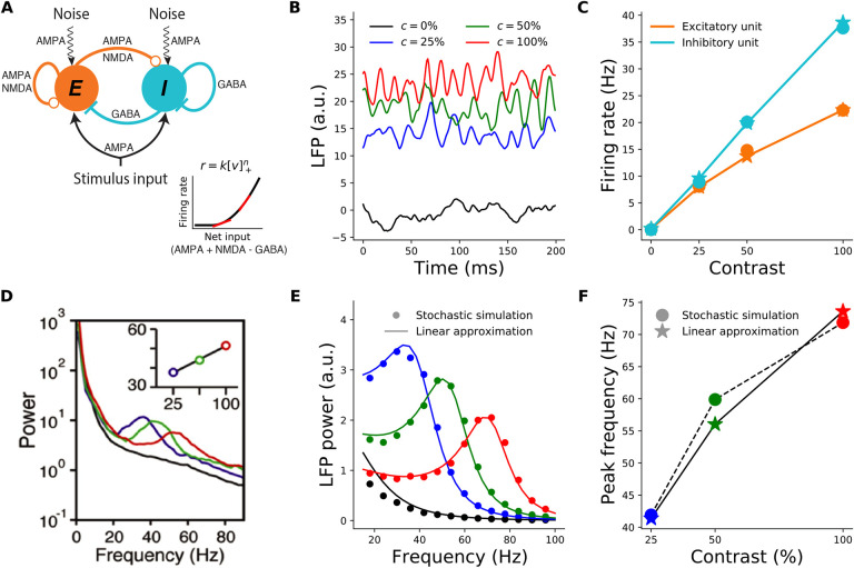
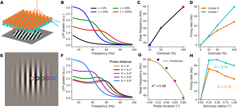
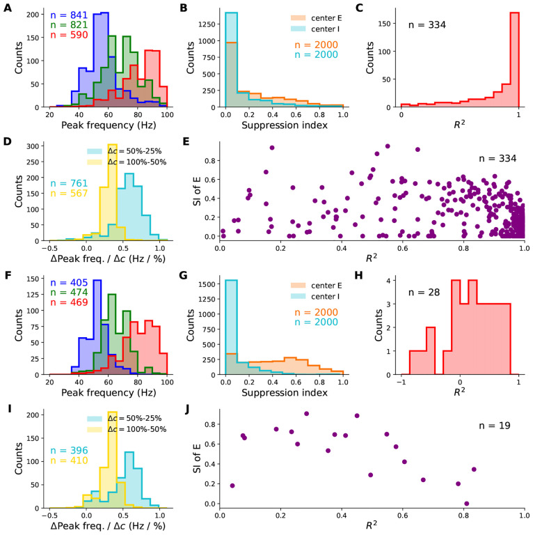
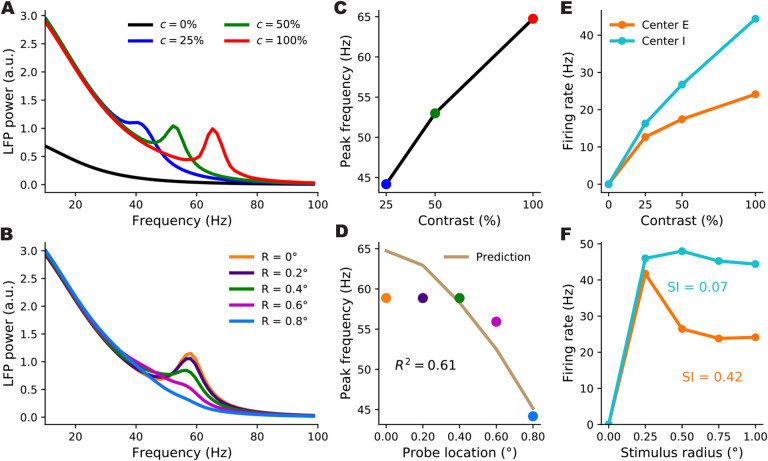
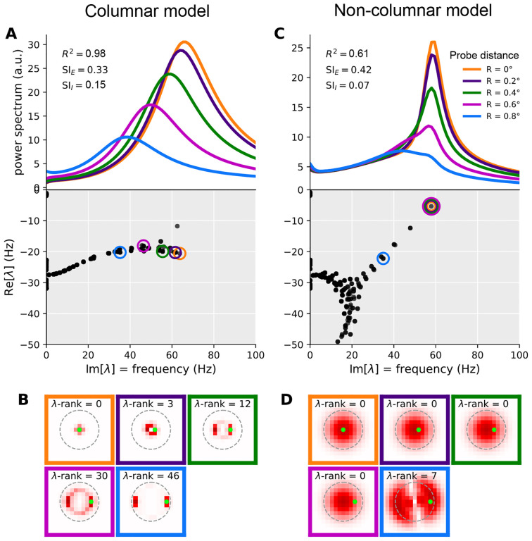
When stimulated, neural populations in the visual cortex exhibit fast rhythmic activity with frequencies in the gamma band (30-80 Hz). The gamma rhythm manifests as a broad resonance peak in the power-spectrum of recorded local field potentials, which exhibits various stimulus dependencies. In particular, in macaque primary visual cortex (V1), the gamma peak frequency increases with increasing stimulus contrast. Moreover, this contrast dependence is local: when contrast varies smoothly over visual space, the gamma peak frequency in each cortical column is controlled by the local contrast in that column's receptive field. No parsimonious mechanistic explanation for these contrast dependencies of V1 gamma oscillations has been proposed. The stabilized supralinear network (SSN) is a mechanistic model of cortical circuits that has accounted for a range of visual cortical response nonlinearities and contextual modulations, as well as their contrast dependence. Here, we begin by showing that a reduced SSN model without retinotopy robustly captures the contrast dependence of gamma peak frequency, and provides a mechanistic explanation for this effect based on the observed non-saturating and supralinear input-output function of V1 neurons. Given this result, the local dependence on contrast can trivially be captured in a retinotopic SSN which however lacks horizontal synaptic connections between its cortical columns. However, long-range horizontal connections in V1 are in fact strong, and underlie contextual modulation effects such as surround suppression. We thus explored whether a retinotopically organized SSN model of V1 with strong excitatory horizontal connections can exhibit both surround suppression and the local contrast dependence of gamma peak frequency. We found that retinotopic SSNs can account for both effects, but only when the horizontal excitatory projections are composed of two components with different patterns of spatial fall-off with distance: a short-range component that only targets the source column, combined with a long-range component that targets columns neighboring the source column. We thus make a specific qualitative prediction for the spatial structure of horizontal connections in macaque V1, consistent with the columnar structure of cortex.

Figure 1.

Contrast dependence of the gamma peak frequency in the 2-population model. A: Schematic of the 2-population Stabilized Supralinear Network (SSN). Excitatory (E) connections end in a circle; inhibitory (I) connections end in a line. Each unit represents a sub-population of V1 neurons of the corresponding E/I type. Both receive inputs from the stimulus, as well as noise input. Inset: The rectified power-law Input/Output transfer function of SSN units (black). Red lines indicate the slope of the I/O function at particular locations. B: Local field potential (LFP) traces, modeled as total net input to the E unit, from the stochastic model simulations under four different stimulus contrasts (c): 0% (black) equivalent to no stimulus or spontaneous activity, 25% (blue), 50% (green), 100% (red). The same color scheme for stimulus contrast is used throughout the paper. (Note that we take stimulus strength (input firing rate) to be proportional to contrast, although in reality it is monotonic but sublinear in contrast, Kaplan et al., 1987). C: Mean firing rates of the excitatory (orange) and inhibitory (cyan) units as a function of contrast, from the stochastic simulations (dots) and the noise-free approximation of the fixed point, Eq. (3) (stars). Note that the dots and stars closely overlap. D: Reproduction of figure 1I from (Ray and Maunsell, 2010) showing the average of experimentally measured LFP power-spectra in Macaque V1. The inset shows the dependence of gamma peak frequency on the contrast of the grating stimulus covering the recording site’s receptive field. E: LFP power-spectra for c = 0%, 25%, 50%, 100% (black, blue, green, and red curves, respectively) calculated from the noise-driven stochastic SSN simulations (dots), or using the linearized approximation (solid lines). F: Gamma peak frequency as a function of contrast, obtained from power-spectra calculated using stochastic simulations (dots and dashed line) or the linearized approximation (stars and solid line).

Figure 2.

Robustness of the contrast-dependence of gamma peak frequency to network parameter variations. One thousand 2-population SSN’s were simulated with randomly sampled parameters (but conditioned on producing stable noise-free steady-states), across wide biologically plausible ranges. All histograms show counts of sampled networks; the total numbers (n’s) vary across different histograms, as different subsets of network produced the corresponding feature or value in the corresponding condition (e.g., a gamma peak at 50% contrast). Panels A-E and F-J show results for the columnar and non-columnar models, respectively. A: Distributions of the excitatory unit’s firing rate in response to 25%, 50%, and 100% contrast stimuli (blue, green, red), plotted on a logarithmic scale. 100% of networks shown across all contrasts. B: Distributions of the gamma peak frequencies at different stimulus contrasts. The n’s (upper right) give the number of networks with a power spectrum peak above 20 Hz. C: Distributions of the gamma peak widths at different stimulus contrasts. D: Same as panel A, but for the inhibitory unit. E: Distributions of the change in gamma peak-frequency normalized by the change in stimulus contrast, either 25% and 50% (cyan) or 50% and 100% (yellow). F: Same as panel E, but for gamma peak-width.

Figure 3.

The supralinear nature of the neural transfer function can explain the contrast dependence of gamma frequency. A: Schematic diagrams of the 2-population SSN (see Fig. 1A) receiving a low (left) or high (right) contrast stimulus. The thickness of connection lines represents the strength of the corresponding effective connection weight, which is the product of the anatomical weight and the input/ouput gain of the presynaptic neuron. The gain is the slope (red line) of the neural supralinear transfer function (black curve), shown inside the circles representing the E (orange) and I (cyan) units. A resonance frequency exists when the effective “negative feedback” (gray arrow enlcosing a minus sign) dominates the effective “positive feedback” (gray arrows enclosing positive signs), in the sense of the inequality Eq. (8). As the stimulus drive (c) increases (right panel), the neurons’ firing rates at the network’s operating point increase. As the transfer function is supralinear, this translates to higher neural gains and stronger effective connections. When a resonance frequency already exists at the lower contrast, this strengthening of effective recurrent connections leads to an increase in the gamma peak frequency, approximately given by the imaginary part of the linearized SSN’s complex eigenvalue, Eq. (6). B: The eigenvalue formula (9) provides an excellent approximation to the gamma peak frequency across sampled networks and contrasts simulated in Fig. 2; correlation coefficient =0.98 (p < 10⁻⁶), for all data points combined across 25% (blue), 50% (green), and 100% (red) contrasts. C: The negative feedback loop contribution to the resonance frequency (Eq. (9) with the second term under the square root neglected) overestimates gamma peak frequency but is positively and significantly correlated with it; correlation coefficient =0.67(p < 10⁻⁶).

Figure 4.

A retinotopically-structured SSN model of V1, with a boost to local, intra-columnar excitatory connectivity, exhibits a local contrast-dependence of gamma peak frequency, as well as robust surround suppression of firing rates. A: Schematic of the model’s retinotopic grid, horizontal connectivity, and stimulus inputs. Each cortical column has an excitatory and an inhibitory sub-population (orange and cyan balls) which receive feedforward inputs (green arrows) from the visual stimulus, here a grating, according to the column’s retinotopic location. Orange lines show horizontal connections projecting from two E units; note boost to local connectivity represented by larger central connection. Inhibitory connections (cyan lines) only targeted the same column, to a very good approximation. B: LFP power-spectra in the center column evoked by flat gratings of contrasts 25% (blue), 50% (green), and 100% (red). C: Gamma peak frequency as a function of flat grating contrast. Note that peaks were defined as local maxima of the relative power-spectrum, i.e., the point-wise ratio of the absolute power-spectrum (as shown in B), to the power-spectrum at zero contrast; see Methods. D: Firing rate responses of E (orange) and I (cyan) center sub-populations as a function of grating contrast. E: The Gabor stimulus with non-uniform contrast (falling off from center according to a Gaussian). The colored circles show the five different cortical locations (retinotopically mapped to the visual field) probed by the LFP “electrodes”. The orange probe was at the center and the distance between adjacent probe locations was 0.2° of visual angle (corresponding to 0.4 mm in V1, the width of the model columns). F: LFP power-spectra evoked by the Gabor stimulus at different probe locations (legend shows the probe distances from the Gabor center). G: Gamma peak frequency of the power-spectra at increasing distance from the Gabor center. The golden curve is the prediction for peak frequency in the displaced probe location based on the Gabor contrast in that location and the gamma peak frequency obtained in the center location for the flat grating of the same contrast. The predictor’s fit to actual Gabor frequencies is very tight (R²=0.98), exhibiting local gamma contrast dependence. H : Size tuning curves of the center E (orange) and I (cyan) subpopulations, at full contrast. E and I firing rates vary non-monotonically with grating size and exhibit surround suppression (suppression indices were 0.33 and 0.15, respectively.

Figure 5.

Behaviour of retinotopic V1 models with and without boosted intra-columnar recurrent excitatory connectivity (columnar vs. non-columnar models, respectively) across their parameter space. We simulated 2000 different networks of each type with parameters (11 in total) randomly sampled across wide, biologically plausible ranges. All histograms show counts of sampled networks; the total number of samples vary across histograms, as only subsets of networks exhibited the corresponding feature with a value in the shown range. Panels A-E and F-J show results for the columnar and non-columnar models, respectively. A & F: Distributions of gamma peak frequency, recorded at stimulus center, for different contrasts of the uniform grating (histograms for 25%, 50%, and 100% contrasts in blue, green and red, respectively). D & I: Distributions of the change in gamma peak-frequency normalized by the change in grating contrast, changing from25% to 50% (cyan) or from 50% to 100% (yellow). B & G: Distributions of the suppression index for the center E (orange) and I (cyan) sub-populations. C & H : The distributions of the coefficient of variation R², as a measure of the locality of gamma peak contrast dependence. The R² quantifies the goodness-of-fit of predicted gamma peak frequency based on local Gabor contrast (see Fig. 4G showing such a fit in an example network). E & J: The joint distribution of R² and the suppression index of the center E sub-population. Only a very small minority of sampled non-columnar networks produced R² > −1 and R² > 0 to appear in H and; hence the small n’s, corresponding to 1.4% and 1% of samples, respectively

Figure 6.

Gamma peak contrast dependence and surround suppression in an example non-columnar retinotopic SSN without a boost in intra-columnar E-connections. Panel descriptions are the same as for the right three columns in Fig. 4. Among 2000 sampled non-columnar networks, this network was the best sample we found in terms of capturing the local contrast dependence of gamma peak frequency (subject to having a nonzero suppression index, and producing realistic non-multiple gamma peaks in the LFP power-spectra which are not unbiologically sharp). However, as seen in panel D, this network only yielded an R² of 0.61, as an index of locality for the gamma peak’s contrast dependence, and gamma peak frequency stayed roughly constant over most of the area covered by the Gabor stimulus (panel B).

Figure 7.

Mechanism of local contrast dependence in the retinotopic SSN with columnar structure and its failure in the non-columnar model. The left and right columns correspond to the columnar (retinotopic SSN with boosted local, intra-columnar excitatory connectivity) and non-columnar (retinotopic SSN without the boost in local connectivity) example networks in Fig. 4 and Fig. 6, respectively. A: Top: relative LFP power spectra recorded at different probe locations in the Gabor stimulus condition (see 4E; same colors are used here to denote the different LFP probes). Relative power spectrum is the point-wise ratio of the evoked power spectrum (evoked by the Gabor stimulus) to the spontaneous power spectrum in the absence of visual stimulus (the absolute power spectrum for the same conditions was given in Fig. 4F). Bottom: the eigenvalue spectrum in the complex plane, with real and imaginary axis exchanged so that the imaginary axis aligns with the frequency axis on top (eigenvalues are also scaled by 1/(2π) to correspond to non-angular frequency). The eigenvalues were weighted separately for each probe, according to Eq. 11, and the eigenvalue with the highest weight was circled with the probe’s color (see 4E). This eigenvalue contributes the strongest peak to the power spectrum at that probe’s location. B: Each sub-panel corresponds to one of the probe locations (as indicated by the frame color), and plots the absolute value of the highest-weight eigenvector (more precisely, the function |ℛ_a(x)| defined in Eq. (37)) over cortical space. Thus, this is the eigenvector corresponding to the circled eigenvalue in panel A, bottom. The λ-rank in each sub-panel is the order (counting from 0) of the eigenvalue according to decreasing imaginary part, which is the eigen-mode’s natural frequency. The green dot in each sub-panel shows the location of the LFP probe. C-D: Same as A and B, but for the retinotopic SSN model with no columnar structure.

References

1. Adesnik H. (2017). Synaptic Mechanisms of Feature Coding in the Visual Cortex of Awake Mice. Neuron, 95:1147–1159. - PMC - PubMed
1. Ahmadian Y. and Miller K. D. (2021). What is the dynamical regime of cerebral cortex? Neuron, 109(21):3373–3391. - PMC - PubMed
1. Ahmadian Y., Rubin D. B., and Miller K. D. (2013). Analysis of the stabilized supralinear network. Neural Computation, 25(8):1994–2037. - PMC - PubMed
1. Anderson J., Lampl I., Gillespie D., and Ferster D. (2000). The contribution of noise to contrast invariance of orientation tuning in cat visual cortex. Science (New York, NY), 290(5498):1968–1972. - PubMed
1. Barbieri F., Mazzoni A., Logothetis N. K., Panzeri S., and Brunel N. (2014). Stimulus dependence of local field potential spectra: Experiment versus theory. Journal of Neuroscience, 34(44):14589–14605. - PMC - PubMed
Publication types