Insights from a genome-wide truth set of tandem repeat variation

Abstract

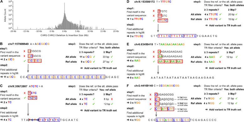
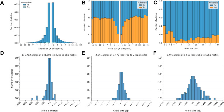
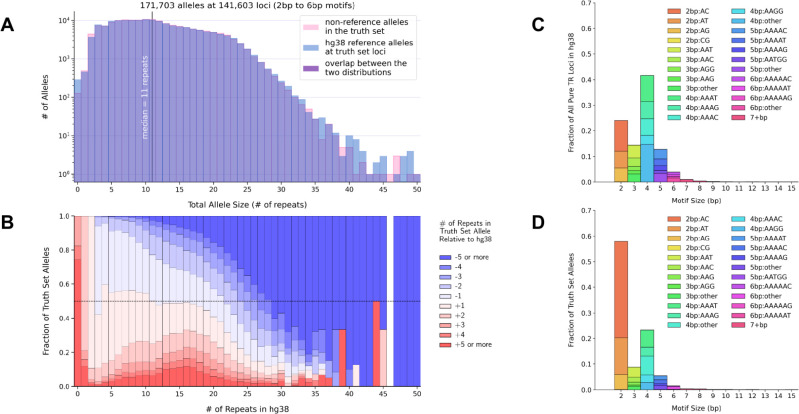
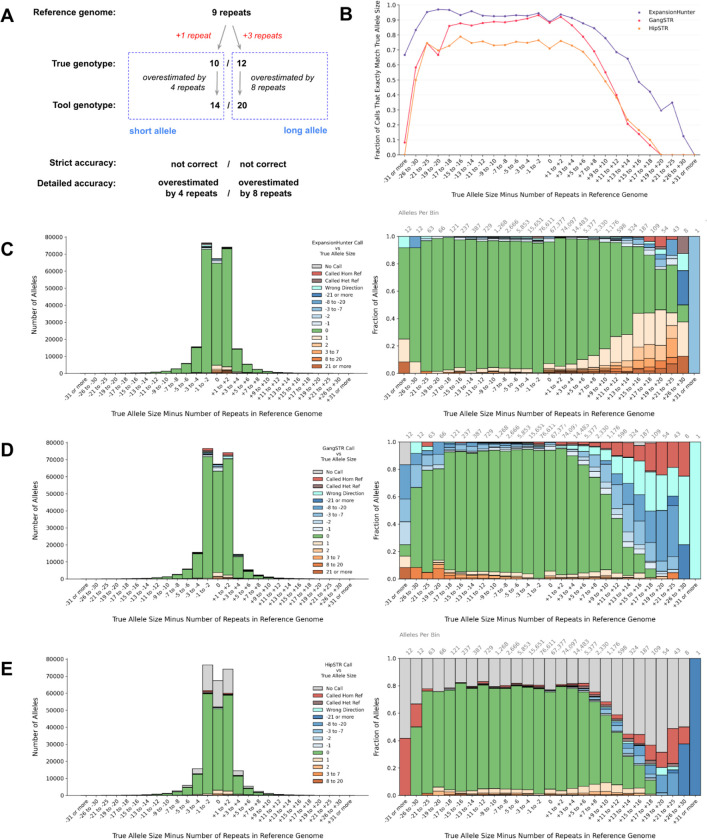
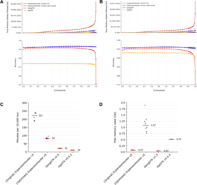
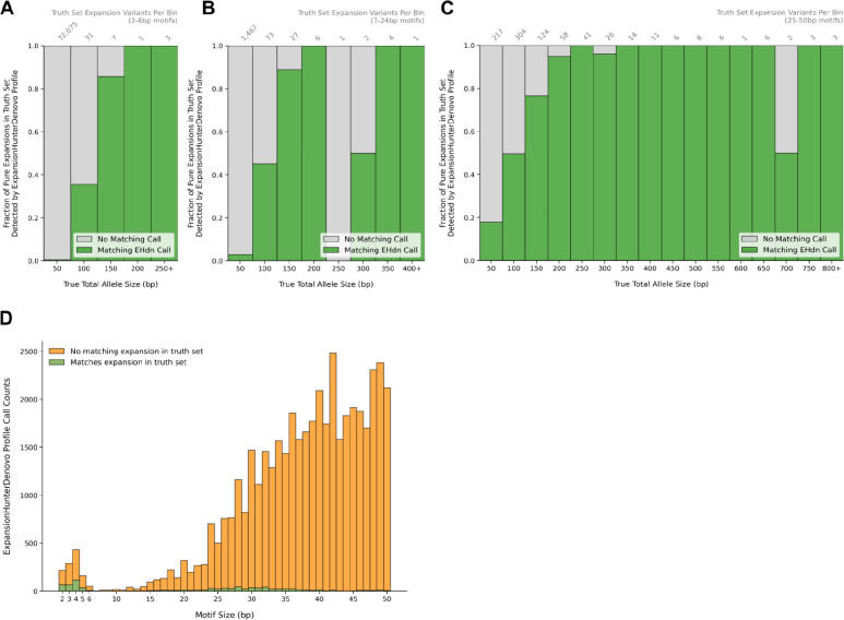
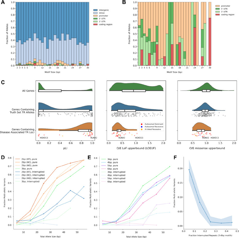
Tools for genotyping tandem repeats (TRs) from short read sequencing data have improved significantly over the past decade. Extensive comparisons of these tools to gold standard diagnostic methods like RP-PCR have confirmed their accuracy for tens to hundreds of well-studied loci. However, a scarcity of high-quality orthogonal truth data limited our ability to measure tool accuracy for the millions of other loci throughout the genome. To address this, we developed a TR truth set based on the Synthetic Diploid Benchmark (SynDip). By identifying the subset of insertions and deletions that represent TR expansions or contractions with motifs between 2 and 50 base pairs, we obtained accurate genotypes for 139,795 pure and 6,845 interrupted repeats in a single diploid sample. Our approach did not require running existing genotyping tools on short read or long read sequencing data and provided an alternative, more accurate view of tandem repeat variation. We applied this truth set to compare the strengths and weaknesses of widely-used tools for genotyping TRs, evaluated the completeness of existing genome-wide TR catalogs, and explored the properties of tandem repeat variation throughout the genome. We found that, without filtering, ExpansionHunter had higher accuracy than GangSTR and HipSTR over a wide range of motifs and allele sizes. Also, when errors in allele size occurred, ExpansionHunter tended to overestimate expansion sizes, while GangSTR tended to underestimate them. Additionally, we saw that widely-used TR catalogs miss between 16% and 41% of variant loci in the truth set. These results suggest that genome-wide analyses would benefit from genotyping a larger set of loci as well as further tool development that builds on the strengths of current algorithms. To that end, we developed a new catalog of 2.8 million loci that captures 95% of variant loci in the truth set, and created a modified version of ExpansionHunter that runs 2 to 3x faster than the original while producing the same output.

Figure 1:. Deriving a TR truth set from the Synthetic Diploid Benchmark

A. Ins/del allele size distribution in the synthetic diploid benchmark. A histogram of allele sizes for all 562,891 deletions and insertions found within SynDip high-confidence regions. On the x axis, positive values represent insertion sizes, while negative values represent deletion sizes in kilobases. B. Example 1: How the TR filter determines if an insertion represents a TR expansion. To decide whether the A > AGCGGCG 6bp insertion in SynDip at position chr7:157009949 is a pure tandem repeat variant, the filter first uses brute force k-mer search on just the GCGGCG variant sequence to find that it consists of 2 x GCG repeats. Then, in step 2, it looks for additional GCG repeats in the reference immediately to the left and right of the insertion point and finds 9 more repeats there. Since there are 11 total GCG repeats spanning 33 base pairs, this insertion passes the filter criteria (≥3 repeats and spanning ≥9 bp) and is included in the truth set as a TR expansion with a true allele size of 11 x GCG repeats and locus coordinates chr7:157009950–157009976. C. Example 2: How the TR filter determines if a deletion represents a TR contraction. To decide whether this 4bp deletion is a pure TR variant, the filter first finds that the deleted bases consist of 2 x TC repeats and then finds 4 additional TC’s in the reference immediately to the right of the deletion. It concludes that the allele is a TR contraction with a true allele size of 4 x TC and locus coordinates chrX:35672888–35672899. D. Example 3: No repeats in the variant sequence. When the filter finds that it can’t divide the variant sequence into pure repeats of a smaller motif, it takes the motif to be the entire variant sequence. Then, it checks the reference context and finds 3 more TTGTC’s there. This allele is then added to the truth set as 4 x TTGTC at locus chrX:153586173–153586188 because it has ≥ 3 repeats and spans ≥ 9bp overall. E. Example 4: No adjacent repeats in the reference context. Since the filter starts with the variant sequence in step 1, it is able to detect TRs even when they have no matching repeats in their immediate reference context. In this example, there are 4 x AAG repeats in the variant sequence and none immediately to the left or right of the insertion point. The 4 x AAG repeats pass the filter criteria of having ≥ 3 repeats and spanning ≥ 9bp. Alternatively, this example could reasonably be considered an interrupted repeat with an AAN motif that has at least 8 matching repeats in the reference sequence. However, because the filter implementation only tests a variant for interrupted repeats if it doesn’t pass the filtering criteria as a pure repeat, this variant is added to the truth set as a pure non-reference allele with 4 x AAG repeats. F. Example 5: Detecting TRs that have interruptions. When the filter determines that an ins/del variant doesn’t pass thresholds as a pure tandem repeat, it retests the sequence, but this time allowing one position to vary across repeats of the motif. In step 1 of this retest phase, it performs a brute force search to find that the variant sequence consists of 3 repeats of an NGG motif where the first position varies across repeats. In step 2, it extends the repeats into the reference context and finds 4 additional NGG repeats. It then adds this allele to the truth set as a 7 x NGG allele at locus chr2:44169141–44169152.

Figure 2:. Allele size distribution

A. Distribution of TR allele sizes. The x axis shows truth set allele sizes minus the number of repeats in hg38 so that expansions relative to the reference are represented as positive numbers and contractions as negative numbers. The y axis shows the fraction of alleles that fall into each size bin. Darker blue represents pure repeats and light blue represents repeats with interruptions. Heterozygous reference alleles (size = +0) are not plotted. B. Fraction of multi-allelic variants by allele size. As in panel A, the x-axis represents true allele sizes relative to the reference. Orange represents the fraction of alleles that occur within multi-allelic loci. These are TR loci where both alleles differ from the hg38 reference and from each other. C. Fraction of multi-allelic variants by motif size. The x axis represents TR motif sizes ranging from 2 to 24bp. The y axis shows, for each motif size, the fraction of alleles that occurs at multi-allelic loci. This plot does not include the 1,746 alleles with motif sizes between 25–50bp. D. Size distribution of alleles with 2–6bp motifs. The x axis shows total allele size in base pairs, including any repeats found in the reference genome at each locus. The y axis is log-scale and shows the total number of alleles in each size bin. E. Size distribution of alleles with 7–24bp motifs. Same as in panel D. F. Size distribution of alleles with 25–50bp motifs. Same as in panel D.

Figure 3:. TR allele and motif sizes compared to repeat sequences in hg38

A. Truth set allele sizes vs reference allele sizes at truth set loci with 2–6bp motifs. The x axis shows allele sizes in terms of numbers of repeats. The y axis counts how many alleles of the given size (x axis) were found among truth set non-reference alleles (pink) or among hg38 reference alleles at truth set loci (blue). The two distributions are plotted on top of each other using semi-transparent colors so that their overlap appears purple. The vertical line at x = 11 indicates the median number of repeats, which has the same value for both distributions. For the blue distribution, the reference allele size is counted twice at multi-allelic loci so that the two distributions have the same number of counts. B. Reference repeat sizes with 2–6bp motifs vs size of expansion or contraction at that locus. This plot shows, for each reference locus size bin, what fraction of truth set alleles were expansions or contractions relative to the reference. The x axis is the same as in panel A. The y axis represents the fraction of the total number of alleles in each size bin. Colors show truth set allele sizes relative to the number of repeats in the reference. Darker red represents larger expansions while darker blue represents larger contractions. The horizontal dashed black line indicates where y = 0.5. C. Motif size distribution in hg38. For all pure repeat loci in the hg38 reference sequence that span 12 or more base pairs, this plot shows the frequency of different motif sizes and normalized motifs. Motif normalization involves taking the motif sequence and its reverse complement, computing all possible cyclic shifts of these sequences, and then selecting the cyclic shift that is alphabetically first, so that, for example, CAT, GAT, and TGA would all be normalized to ATC. The x axis represents motif sizes in base pairs. The y axis represents the fraction of all loci that have a given motif size. Colors distinguish the most frequently occurring normalized motifs within each motif size bin. D. Motif size distribution in the truth set. Motif sizes of all TR alleles in the truth set, shown using the same axes and colors as panel C.

Figure 4:. ExpansionHunter, GangSTR, and HipSTR accuracy for pure repeats with 2–6bp motifs at 30x read depth

A. Schematic for quantifying a tool’s accuracy at a single TR locus. When evaluating a tool’s genotype at a particular locus, there are 5 numbers to consider: the number of repeats in the reference, the two allele sizes in the truth set, and the two allele size estimates produced by the tool. In this example, the reference locus contains 9 repeats. The SynDip TR variant at the locus is multi-allelic, with the shorter allele being an expansion by +1 repeat, while the longer allele is an expansion by +3 repeats. The true genotype is therefore 10 / 12 repeats. A hypothetical TR genotyping tool estimates the genotype as 14 / 20 repeats. To quantify the accuracy of this call, we compare the tool’s long allele size with the true long allele size, and the tool’s short allele size with the true short allele size. We then define strict accuracy as whether the tool exactly matched the true allele size, and detailed accuracy as the integer difference between the tool’s estimated allele size and the true allele size. Panel B compares tools based on strict accuracy. Panels C-E use color to show detailed accuracy (for this example, the colors would be based on the numbers in the dashed blue box). In all panels, the x axis defines bins based on the difference between the true allele size and the number of repeats in the reference (labeled in red). B. Strict accuracy by allele size. The x axis represents true allele sizes relative to the reference. The y axis represents the fraction of alleles that each tool got exactly right. C. ExpansionHunter detailed accuracy by allele size. The x axis represents true allele sizes relative to the reference. The color scale represents detailed accuracy. Green indicates that the tool exactly matched the true allele size and represents the same fraction of calls as those shown in panel B. Orange represents alleles that the tool overestimated, with darker orange indicating larger errors. Blue represents underestimated alleles with darker blue indicating larger underestimates. Teal indicates that the tool called a contraction when the true allele was an expansion, or vice versa. Brown means the tool incorrectly called an allele as heterozygous reference. Red indicates when the tool called a variant locus as homozygous reference and so entirely missed the variant. Finally, gray represents loci where the tool didn’t produce a genotype (i.e. due to errors or insufficient coverage). The left-side plot shows total allele counts on the y axis while the right-side plot shows the same information but normalizing each bin to 100% and showing the fraction of alleles on the y axis. The total number of loci represented within each bar is also labeled above the right-side plot. D. GangSTR detailed accuracy by allele size. Axes and colors defined as in panel C. E. HipSTR detailed accuracy by allele size. Axes and colors defined as in panel C.

Figure 5:. Genotype quality filters and tool performance for pure repeats with 2–6bp motifs at 30x read depth

A. Tool performance after post-filtering using different quality score thresholds. This plot shows how different minimum quality score thresholds affect post-filtering accuracy for calls on truth set loci with pure repeats of 2–6bp motifs and short read data with 30x coverage. The top panel shows the false negative rate, calculated as the total number or fraction (y-axis) of strictly accurate alleles that didn’t pass a given minimum quality score threshold (x-axis). The bottom panel shows the accuracy (y-axis) of alleles at each quality score threshold (x-axis). Here, accuracy is defined as (true positive alleles + true negative alleles)/(total alleles) and computed as follows: True positive alleles: the tool’s reported allele size exactly equals the true allele size and has a quality score above the minimum threshold True negative alleles: the tool’s reported allele size doesn’t equal the true allele size and has a quality score below the minimum threshold Total alleles: the total number of alleles, including those above and below the quality score threshold For GangSTR and HipSTR, the plot uses quality scores provided by the tools. Since ExpansionHunter doesn’t output a single quality score, the plot shows two different quality scores computed based on ExpansionHunter output: Q from CIs = 1/exp(4 * (confidence interval size)/(called allele size)) as in EnsembleTR Q from reads = the fraction of reads that support the allele size vs. all allele sizes considered by ExpansionHunter at the given locus. This is computed from fields in ExpansionHunter’s json output for each locus. B. Tool performance excluding no-call loci. This plot shows the same metrics as panel A after excluding loci where one or more tools did not produce a genotype. C. Tool runtime per 10,000 loci. The x axis indicates the two versions of ExpansionHunter being compared - the original Illumina version 5 and our optimized version - as well as the versions of GangSTR and HipSTR. The y axis measures runtime in minutes per 10,000 loci. For each tool, runtimes are computed for 8 different batches of truth set variant loci, with each dot representing one batch. The red lines and numerical labels indicate the median runtime across batches. D. Memory usage. The y axis shows peak memory usage in gigabytes for each tool. Dots represent the same 8 batches as used in panel C. Memory usage for ExpansionHunter (both the original and the optimized versions) is based on processing 500 loci per run, and may be higher for larger batches. Red lines and numerical labels indicate the median across batches.

Figure 6:. ExpansionHunterDenovo accuracy

A. Truth set variants detected by the EHdn profile stage: 2–6bp motifs. This plot estimates the sensitivity of ExpansionHunterDenovo’s initial “profile” stage by showing what fraction of pure repeat expansions from the truth set have a matching interval reported by EHdn. Here, an EHdn interval is considered as matching a truth set expansion if they are within 600bp of each other and have the same normalized motif. Panel A only includes truth set variants with motif sizes between 2–6bp. The x axis shows the total allele size of the truth set allele, counting the repeats in the reference as well as the variant sequence. For multi-allelic expansions, the x axis represents the size of the longer expansion since ExpansionHunterDenovo is designed to detect the largest alleles. The y axis shows the fraction of truth set variants within each bin. The number of variants represented within each bar is labeled above the plot. As expected, ExpansionHunterDenovo is most sensitive to repeats longer than the read length (150bp). The EHdn calls in this plot were generated using SynDip short read data downsampled to 30x coverage. B. Truth set variants detected by the EHdn profile stage: 7–24bp motifs. Same as Panel A, but only including truth set variants with motif sizes 7–24bp. C. Truth set variants detected by the EHdn profile stage: 25–50bp motifs. Same as Panel A, but only including truth set variants with motif sizes 25–50bp. D. Specificity of the EHdn profile stage. This plot estimates the specificity of ExpansionHunterDenovo’s “profile” stage by showing how many of its output intervals have a matching expansion variant in the truth set (green) including both pure and interrupted repeats, or no matching variants in the truth set (orange). As in panel A, an EHdn interval is considered as matching a truth set expansion if they are within 600bp of each other and have the same normalized motif. The x axis represents motif sizes. It shows that this initial stage of ExpansionHunterDenovo outputs many repeats that can be considered false positives, especially for larger motif sizes, leaving it to the downstream outlier detection stages to discriminate between true and false positive calls.

Figure 7:. Genome-wide properties of tandem repeat variation

A. Tandem repeats in annotated genomic regions. This plot shows where the truth set’s pure TR variants occur relative to gene regions annotated in MANE v1. The x axis shows TR motif sizes in base pairs. The y axis shows the fraction of alleles in each bin. Colors represent the different annotated regions. B. Tandem repeats in coding regions, UTRs, promoters. Shows the same information as panel A, but excludes TR loci in intronics and intergenic regions in order to more clearly see the fractions for the remaining regions. C. Gene constraint metrics vs genes that contain coding TR variants. This plot shows 3 different measures of gene constraint on the x axis: pLI and LOEUF, and missense constraint. Above the x axis, it displays the constraint score distributions for three different sets of genes: all 19,704 genes with known constraint scores in green, 25 genes that contain known monogenic STR loci within their coding regions in orange, and 161 genes that contain pure TR variants from the truth set within their coding regions. Each dot represents a gene. In the middle track, the dot colors represent autosomal dominant (red), autosomal recessive (blue), and X-linked recessive (orange) inheritance modes of pathogenic STR expansions within those genes. Labels indicate the locations of the HOXD13 and RUNX2 genes which contain the two disease-associated STR loci estimated as having high constraint according to the STR-specific constraint score developed in [Gymrek 2017]. D. Relative mutation rate by motif and allele size for 2bp motifs. The x axis represents the true total allele size in base pairs. Orange colors represent pure repeats of different 2bp motifs (normalized so that, for example, AC, CA, GT, TG are all normalized to AC), while blue colors represent interrupted repeats. Also, repeats with 3bp motifs are shown in green for comparison (bright green for pure repeats, and light green for interrupted). The y axis represents the relative mutation rate of each bin as measured by the fraction of alleles that occurred at multi-allelic loci - ie. those where both alleles differ from hg38 and from each other. Each point in the plot represents a bin with no fewer than 20 alleles. Interrupted alleles were included in this plot if no more than 25% of the repeats within the allele sequence had interruptions (differed from other repeats in the sequence at exactly 1 position within the motif). E. Relative mutation rate by motif and allele size for 3–6bp motifs. Same as in panel D except that colors here represent motif sizes between 3–6bp. The brighter version of each color indicates pure repeats while the lighter color indicates interrupted repeats of that motif size. F. Relative mutation rate by fraction of interrupted repeats. The x axis shows the fraction of repeats within a given allele sequence that differ from the most common motif found in that sequence. For example, for an allele sequence consisting of 4 repeats CAG CAG CAT CAG, this fraction would be 0.25 due to the 1 repeat having a CAT motif. Alleles are only included when repeats differ from each other at exactly one position within the motif - such as in the 3rd position in this example. The y axis shows the relative mutation rate of each bin as measured by the fraction of alleles that occur at multi-allelic loci, similar to panel D. Each point in the plot represents a bin with no fewer than 20 alleles. The plot is based on alleles with 3–6bp motifs. The shaded region represents boot-strapped 95% confidence intervals based on variability within each point across 3, 4, 5, and 6bp motif sizes.

References

1. Depienne C, Mandel JL. 30 years of repeat expansion disorders: What have we learned and what are the remaining challenges? Am J Hum Genet. 2021. May 6;108(5):764–85. - PMC - PubMed
1. Brais B. Correction: Short GCG expansions in the PABP2 gene cause oculopharyngeal muscular dystrophy. Nat Genet. 1998. Aug;19(4):404–404. - PubMed
1. Yeetong P, Pongpanich M, Srichomthong C, Assawapitaksakul A, Shotelersuk V, Tantirukdham N, et al. TTTCA repeat insertions in an intron of YEATS2 in benign adult familial myoclonic epilepsy type 4. Brain. 2019. Nov 1;142(11):3360–6. - PubMed
1. Mitra I, Huang B, Mousavi N, Ma N, Lamkin M, Yanicky R, et al. Patterns of de novo tandem repeat mutations and their role in autism. Nature. 2021. Jan;589(7841):246–50. - PMC - PubMed
1. Mojarad BA, Engchuan W, Trost B, Backstrom I, Yin Y, Thiruvahindrapuram B, et al. Genome-wide tandem repeat expansions contribute to schizophrenia risk. Mol Psychiatry. 2022. Sep;27(9):3692–8. - PMC - PubMed
Publication types