Canonical correlation analysis for multi-omics: Application to cross-cohort analysis

Abstract

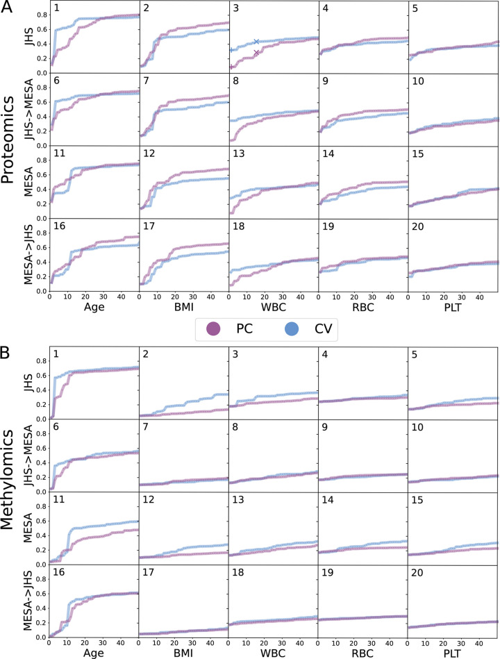
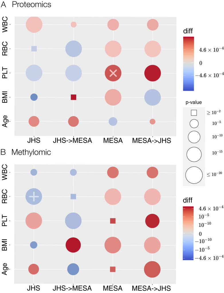
Integrative approaches that simultaneously model multi-omics data have gained increasing popularity because they provide holistic system biology views of multiple or all components in a biological system of interest. Canonical correlation analysis (CCA) is a correlation-based integrative method designed to extract latent features shared between multiple assays by finding the linear combinations of features-referred to as canonical variables (CVs)-within each assay that achieve maximal across-assay correlation. Although widely acknowledged as a powerful approach for multi-omics data, CCA has not been systematically applied to multi-omics data in large cohort studies, which has only recently become available. Here, we adapted sparse multiple CCA (SMCCA), a widely-used derivative of CCA, to proteomics and methylomics data from the Multi-Ethnic Study of Atherosclerosis (MESA) and Jackson Heart Study (JHS). To tackle challenges encountered when applying SMCCA to MESA and JHS, our adaptations include the incorporation of the Gram-Schmidt (GS) algorithm with SMCCA to improve orthogonality among CVs, and the development of Sparse Supervised Multiple CCA (SSMCCA) to allow supervised integration analysis for more than two assays. Effective application of SMCCA to the two real datasets reveals important findings. Applying our SMCCA-GS to MESA and JHS, we identified strong associations between blood cell counts and protein abundance, suggesting that adjustment of blood cell composition should be considered in protein-based association studies. Importantly, CVs obtained from two independent cohorts also demonstrate transferability across the cohorts. For example, proteomic CVs learned from JHS, when transferred to MESA, explain similar amounts of blood cell count phenotypic variance in MESA, explaining 39.0% ~ 50.0% variation in JHS and 38.9% ~ 49.1% in MESA. Similar transferability was observed for other omics-CV-trait pairs. This suggests that biologically meaningful and cohort-agnostic variation is captured by CVs. We anticipate that applying our SMCCA-GS and SSMCCA on various cohorts would help identify cohort-agnostic biologically meaningful relationships between multi-omics data and phenotypic traits.

Fig 1. Cartoon illustration of a typical CCA-based method for three assays.

X, Y, and Z are three assays with 4, 5, and 6 features respectively. When applying a CCA-based method on them to compute 4 canonical variables (CVs), we would first get their weight matrices W_X, W_Y, W_Z, each of which contains 4 weight vectors. By multiplying each assay matrix (left panel) and its corresponding weight matrix (middle panel), we obtain the CV matrix for the assay (right panel) where each column corresponds to one CV.

Fig 2. Improved orthogonality among CVs by adopting the Gram–Schmidt (GS) strategy.

CVs are inferred from MESA proteomics and methylomics data using unsupervised SMCCA. Each row and column represent one CV, ranging from CV1 to CV50. (A-B) Results from the PMA R package, implementation of the original SMCCA methods without the incorporation of GS algorithm. (C-D) Results from our SMCCA-GS, with the GS strategy incorporated. Left panel (A and C) show proteomics CVs, and right panel (B and D) methylomics CVs.

Fig 3. Proportion of variation in outcomes explained by CVs.

(A) CVs were inferred using proteomics and methylomics in JHS. The top 50 CVs were used to calculate the r² (Y-axis) for each outcome (X-axis). (B) We obtained CVs in JHS by applying the weights inferred from MESA, and then calculated r² in the same way as in A. (C) CVs were inferred using proteomics and methylomics in MESA. (D) CVs were obtained in MESA by applying the weights inferred from JHS.

Fig 4. Comparison of r², PCs vs CVs.

Each column corresponds to one outcome. Within each panel, top row (JHS) shows results in JHS using JHS-inferred CVs. Second row (JHS->MESA) shows results in MESA, also using JHS-inferred weights. Third row (MESA) shows results in MESA, this time using MESA-inferred CVs. Last row (MESA->JHS) shows results in JHS, also using MESA-inferred weights. (A) Proteomics. Proteomics CVs explain more variation in white blood cell count (WBC) than PCs. For example, proteomics-CV1 explains 33% of the variation in WBC (blue “+” in Fig 4A3), while proteomics-PC1 only explains 7.7% (purple “+” in Fig 4A3). This pattern persists until approximately 20 CVs/PCs. The top 15 proteomics-CVs in JHS explain 44% of the variation in WBC (blue “×” in Fig 4A3), while the top 15 proteomics-PCs explain only 29% (purple “×” in Fig 4A3). (B) Methylomics. In each sub-figure, X-axis indicates the number of CVs or PCs used and Y-axis the proportion of variation explained in the outcome (i.e., r²).

Fig 5. Comparison of SSCCA and SSMCCA.

(A) proteomics, and (B) methylomics. Each row corresponds to a phenotype (from bottom to top, Age, BMI, WBC, RBC, and PLT). Circle size reflects the significance of the difference in variation explained between two methods. Color reflects the size of difference between the variation of phenotype explained by SSCCA and our SSMCCA. Therefore, a larger circle means a more significant difference between the two methods. Note that we use rectangles for insignificant difference with p > 0.01. Red means that our SSMCCA explains more phenotypic variation while blue means that SSCCA explains more. The darker the color, the larger the difference (the scale is different for parts A and B, annotated in “diff” column on side of figure).