. 2023 Apr 6;3(5):100297.
doi: 10.1016/j.xgen.2023.100297. eCollection 2023 May 10.

Amplification is the primary mode of gene-by-sex interaction in complex human traits

Affiliations

Amplification is the primary mode of gene-by-sex interaction in complex human traits

Carrie Zhu et al. Cell Genom. .

Abstract

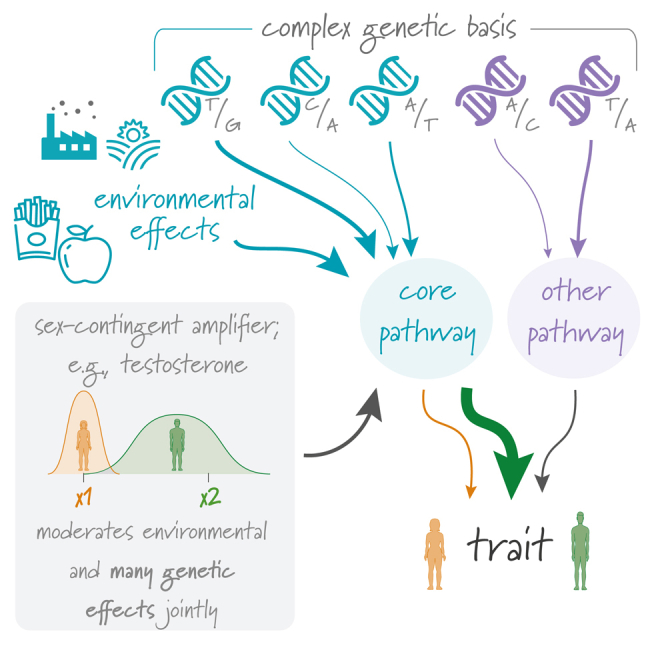
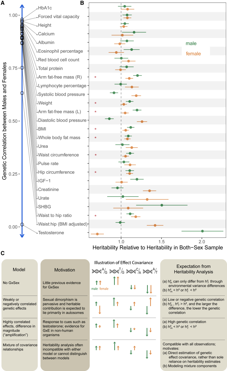
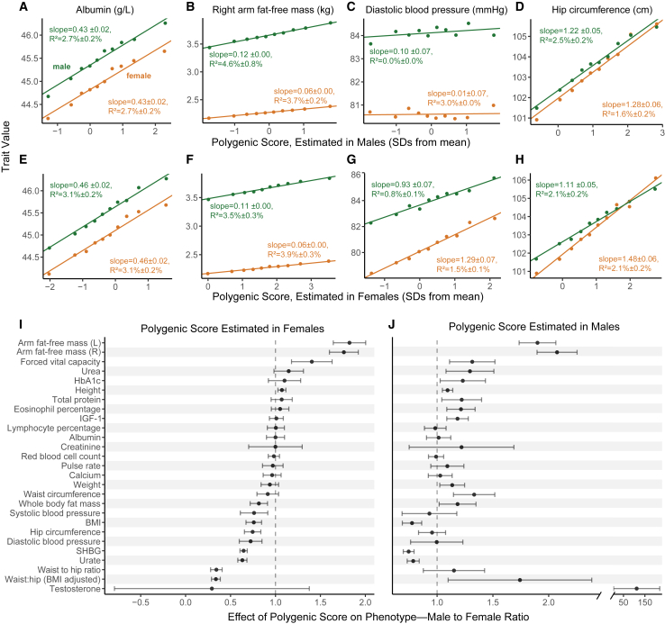
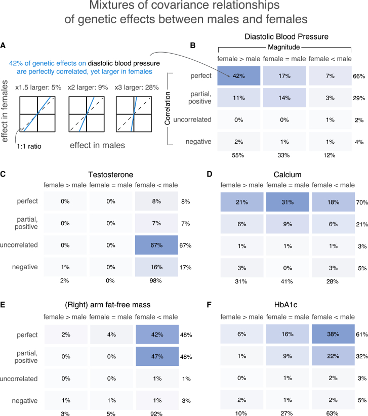
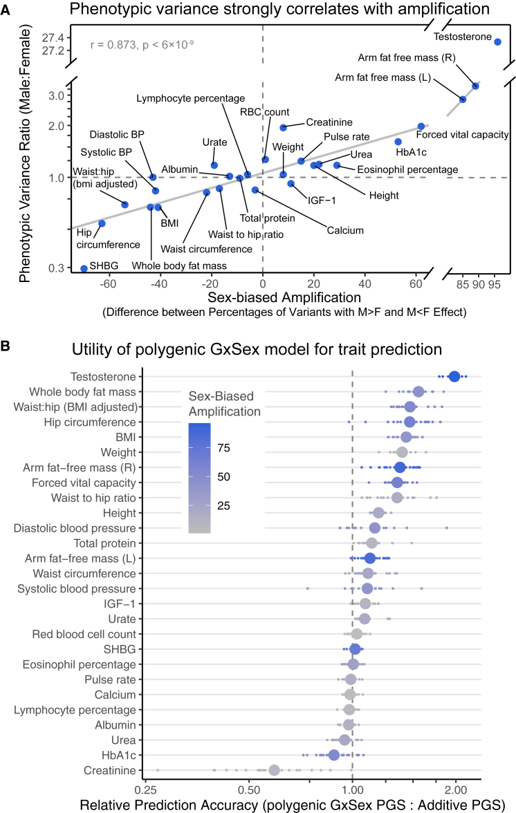
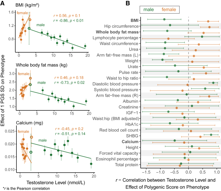
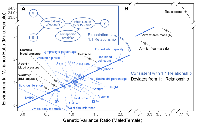
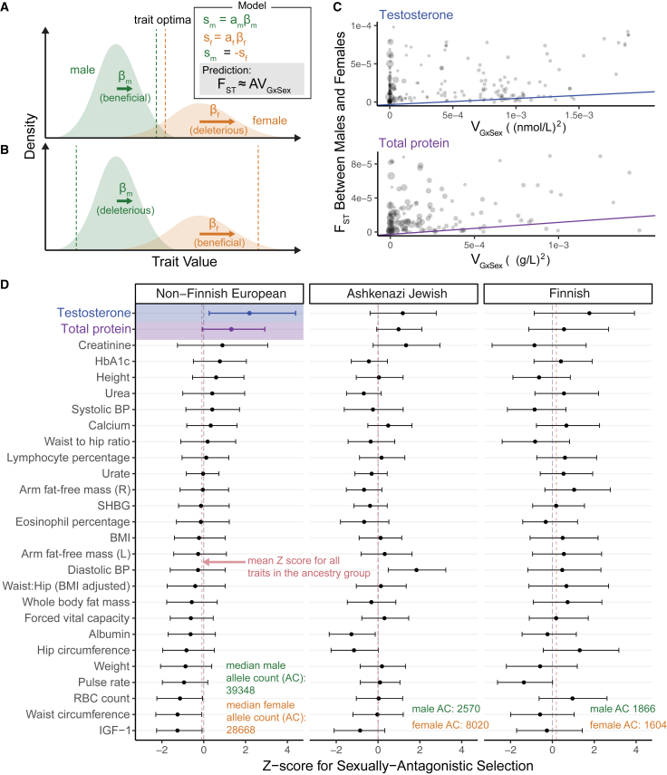
Sex differences in complex traits are suspected to be in part due to widespread gene-by-sex interactions (GxSex), but empirical evidence has been elusive. Here, we infer the mixture of ways in which polygenic effects on physiological traits covary between males and females. We find that GxSex is pervasive but acts primarily through systematic sex differences in the magnitude of many genetic effects ("amplification") rather than in the identity of causal variants. Amplification patterns account for sex differences in trait variance. In some cases, testosterone may mediate amplification. Finally, we develop a population-genetic test linking GxSex to contemporary natural selection and find evidence of sexually antagonistic selection on variants affecting testosterone levels. Our results suggest that amplification of polygenic effects is a common mode of GxSex that may contribute to sex differences and fuel their evolution.


Conflict of interest statement

The authors declare no competing interests.

Figures

None
Graphical abstract
Figure 1
Figure 1
Heritabilities and genetic correlations cannot fully distinguish models of GxSex (A) Genetic correlations between males and females, estimated using bivariate LDSC, are shown in descending order. (B) The x axis represents the relative heritability (i.e., the SNP heritability divided by the SNP heritability) estimated in the sample with both sexes combined. Red asterisks indicate body mass-related traits with greater heritability in both sex-specific samples compared with the sample combining both sexes. Error bars represent ± 1 SE. (C) Polygenic models of GxSex. We examine different models of the nature of GxSex in complex traits that link to previous studies and motivations. Each model leads to different expectations from the analysis of heritability and genetic correlations (A and B). The illustrations in the third column depict examples of directions and magnitudes of genetic effects corresponding to each model. hm2, hf2, and h2 denote narrow-sense heritabilities in males, females, and a combined sample, respectively.
Figure 2
Figure 2
Evaluating evidence of systematic amplification (A–D) We regressed trait values in males (green) and separately in females (orange) on a PGS estimated in an independent sample of males. Points show mean values in one decile of the PGS; the fitted line and associated effect estimate and R2 correspond to regressions on the raw, non-binned data. In some traits, like albumin (A), the PGS has a similar effect on the trait in both sexes. In other traits (B and D), the estimated effect of the PGS differs significantly, consistent with a substantial difference in the magnitude of genetic effects of sites included in the PGS. (E–H) Same analysis as in (A)–(D) but with a PGS pre-estimated in an independent sample of females. (I and J) Summary of the ratio of the effect of the PGS on the trait (±2 SE) in males to the effect in females across physiological traits. See results for other traits in Figure S11.
Figure 3
Figure 3
Polygenic covariance structure between males and females (A) Our analysis of the polygenic covariance between males and females is based on sex-stratified GWASs. We modeled the sex-stratified GWAS estimates as sampled with error from true effects arising from a mixture of possible covariance relationships between female and male genetic effects. As an example, shown are illustrations for three possible relationships of the same qualitative nature—perfectly correlated effects that are also larger in females—and the mixture weights estimated for each in the case of diastolic blood pressure. (B–F) Each box shows the sum of weights placed on all covariance relationships of the same qualitative nature, as specified by relative magnitude (horizontal axis) and correlation (vertical axis) between male and female effects. The full set of pre-specified covariance matrices is shown in Figure S2, and the weights placed on each of them for each trait are shown in Data S1–27. All weights shown are percentages of non-null weights; i.e., the weight divided by the sum of all weights except for the one corresponding to no effect in either sex.
Figure 4
Figure 4
Consequences of amplification for trait variance and polygenic score predictive utility (A) Phenotypic variance strongly correlates with amplification. “Sex-biased amplification” on the x axis is calculated by taking the difference between the sum of mixture weights on covariance matrices with male effects greater in magnitude than female effects (M > F) and the sum of weights of M < F matrices. The solid gray line shows a linear fit across traits, excluding testosterone as an outlier, with correlation summaries in gray in the top left corner. (B) Utility of the polygenic GxSex model for trait prediction. The x axis shows the relative prediction accuracy estimated from the incremental R2 ratio of a GxSex model informed by polygenic covariance patterns and an additive model. For each trait, smaller points show relative prediction accuracies across 20 cross-validation folds, and larger points show the average across the 20 folds. The phenotypes are ordered by the mean relative prediction accuracy. The color of each point corresponds to the degree of sex-biased amplification as described in (A).
Figure 5
Figure 5
Amplification of total genetic effect in relation to testosterone levels (A) The relationship between testosterone level bins and estimated magnitude of genetic effect on traits is shown for three traits. The magnitude of genetic effect is estimated using the slope of the regression of phenotypic values to PGSs in that bin. The units on the y axis are effect per standard deviation (SD) of the PGSs across all individuals in all bins. The hollow data points are bins with overlapping testosterone ranges between males and females; these are based on fewer individuals (∼800 compared with ∼2,200 in other bins) and not included in the regression. Figure S13 show all other traits analyzed. (B) The correlation for each sex (90% CI) are shown for all 27 traits. Traits are ordered in descending order of male-female differences in Pearson correlation.
Figure 6
Figure 6
Testing a model of pervasive, joint amplification of environmental and polygenic effects (A) A model of equal amplification of genetic (G) and environmental (E) effect that produces the sex differences in the distribution of the phenotype, Y. G and E act through a core pathway that is amplified in a sex-specific manner. (B) The blue 1:1 line depicts the theoretical expectation under a simple model of equal amplification of G and E effects in males compared with females. Error bars show 90% confidence intervals. Traits in blue are consistent (within their 90% CI) with the theoretical prediction. Figure S18 shows the same data alongside the predictions under other theoretical models of male-female variance ratios.
Figure 7
Figure 7
Testing for sexually antagonistic selection (A and B) A model of sexually antagonistic selection. Selection coefficients, sm and sf, are linear with the additive effect on the trait in each sex. Sexually antagonistic selection acts so that sm=sf. The model yields the prediction of Equation 1. While in (A), trait optima are close to each other and in (B) they are far apart, in both cases alleles will tend to be antagonistically selected. (C) Two examples of the weighted least-squares linear regression performed to estimate the strength of sexually antagonistic selection on variants associated with a trait (A in A and Equation 1). Each point shows one SNP. Size is proportional to each point’s regression weight. (D) Z scores (90% non-parametric bootstrap CI) estimated through 1,000 resampling iterations of the weighted linear regression of (B) for each trait. The two colored estimates correspond to the examples in (B) and (C).

Similar articles

Cited by

References

    1. van Doorn G.S. Intralocus sexual conflict. Ann. N. Y. Acad. Sci. 2009;1168:52–71. doi: 10.1111/j.1749-6632.2009.04573.x. - DOI - PubMed
    1. Arnqvist G., Rowe L. Princeton University Press; 2005. Sexual Conflict. - DOI
    1. Camus M.F., Piper M.D., Reuter M. Sex-specific transcriptomic responses to changes in the nutritional environment. Elife. 2019;8 doi: 10.7554/eLife.47262. - DOI - PMC - PubMed
    1. Bayer E.A., Stecky R.C., Neal L., Katsamba P.S., Ahlsen G., Balaji V., Hoppe T., Shapiro L., Oren-Suissa M., Hobert O. Ubiquitin-dependent regulation of a conserved DMRT protein controls sexually dimorphic synaptic connectivity and behavior. Elife. 2020;9 doi: 10.7554/eLife.59614. - DOI - PMC - PubMed
    1. Baar E.L., Carbajal K.A., Ong I.M., Lamming D.W. Sex- and tissue-specific changes in mTOR signaling with age in C57 BL/6J mice. Aging Cell. 2016;15:155–166. doi: 10.1111/acel.12425. - DOI - PMC - PubMed

LinkOut - more resources