Examining the impact of dimethyl sulfide emissions on atmospheric sulfate over the continental U.S

Abstract

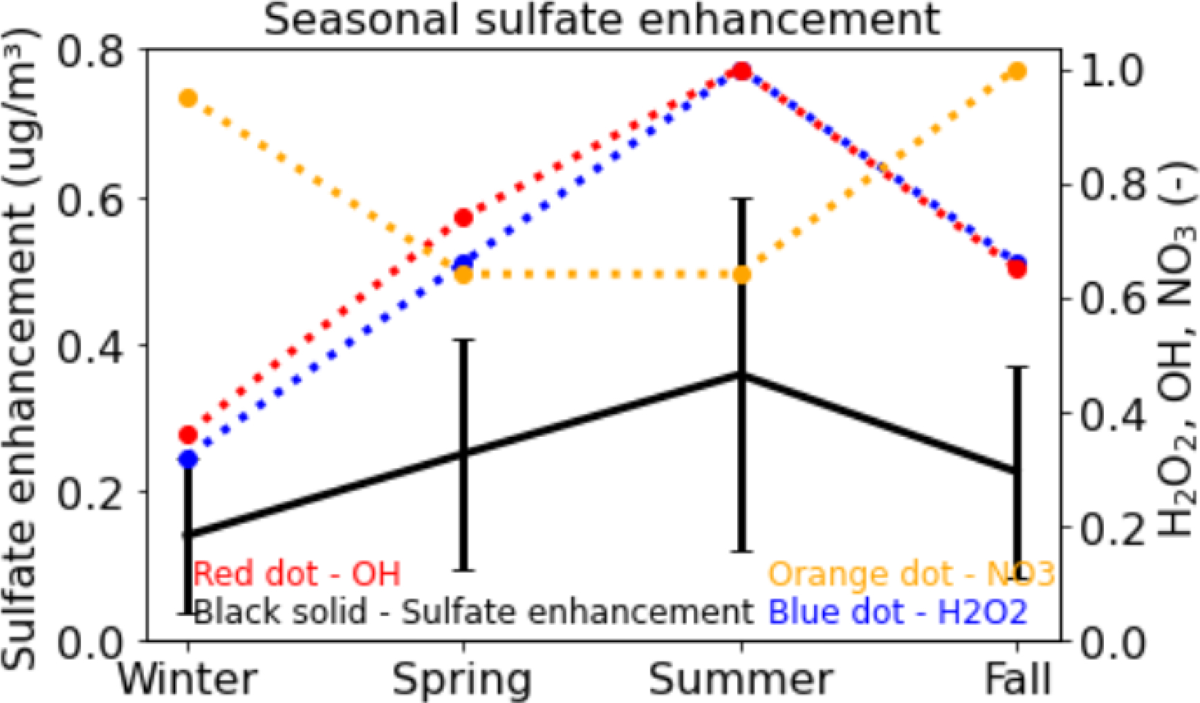
We examine the impact of dimethylsulfide (DMS) emissions on sulfate concentrations over the continental U.S. by using the Community Multiscale Air Quality (CMAQ) model version 5.4 and performing annual simulations without and with DMS emissions for 2018. DMS emissions enhance sulfate not only over seawater but also over land, although to a lesser extent. On an annual basis, the inclusion of DMS emissions increase sulfate concentrations by 36% over seawater and 9% over land. The largest impacts over land occur in California, Oregon, Washington, and Florida, where the annual mean sulfate concentrations increase by ~25%. The increase in sulfate causes a decrease in nitrate concentration due to limited ammonia concentration especially over seawater and an increase in ammonium concentration with a net effect of increased inorganic particles. The largest sulfate enhancement occurs near the surface (over seawater) and the enhancement decreases with altitude, diminishing to 10-20% at an altitude of ~5 km. Seasonally, the largest enhancement of sulfate over seawater occurs in summer, and the lowest in winter. In contrast, the largest enhancements over land occur in spring and fall due to higher wind speeds that can transport more sulfate from seawater into land.

Keywords: CMAQ; DMS; SO2; seawater; sulfate.

Figure 1.

Seasonal DMS emissions over the modeling domain calculated using the Liss and Merlivat [34] parameterization for the water side gas transfer velocity (${\text{k}}_{\text{w}}$). DMS_w, wind speed, and SST values shown on the right y-axis are dimensionless. Normalized values are calculated by dividing the actual values by their maximum values. Winter represents December-February, spring represents March-May, summer represents June-August, and fall represents September-November.

Figure 2.

Predicted annual mean changes (WDMS – NODMS) in surface (a) sulfate, (b) nitrate, (c) ammonium, and (d) total inorganic particle concentrations by DMS emissions. Changes in inorganic particle concentrations are calculated as the net effect due to increases in sulfate and ammonium and decreases in nitrate concentrations.

Figure 3.

Seasonal impacts of DMS emissions on sulfate over seawater. H₂O₂, OH and NO₃ concentrations shown on the right y-axis are dimensionless. Normalized values are calculated by dividing the actual concentrations by their maximum concentrations and are shown on y-axis. Winter represents December-February, spring represents March-May, summer represents June-August, and fall represents September-November. Solid vertical lines represent standard deviation of sulfate enhancement.

Figure 4.

Spatial distribution of the seasonal impacts of DMS emissions on sulfate in (a) winter, (b) spring, (c) summer, and (d) fall. Figure 4(a) shows monitoring locations for observed data used in Figure 8.

Figure 5.

Diurnal variation of the impacts of DMS emissions on sulfate over the Pacific Ocean in July. All grid-cells over the Pacific Ocean (including the Gulf of California) are used for the calculation. Solid vertical lines represent standard deviation of sulfate enhancement.

Figure 6.

Impact of DMS emissions on sulfate aloft. Solid lines represent mean and shaded areas represent standard deviation of sulfate enhancement.

Figure 7.

(a) Combined impact of DMS emissions and boundary conditions on sulfate (b) fractional impact of within-domain DMS emissions on sulfate, and (c) fractional impact of outside-domain DMS emissions (specified through boundary conditions) on sulfate in July..

Figure 8.

A comparison of predicted sulfate without and with DMS emissions to observed sulfate in (a) the Pacific-coast states, (b) the Gulf-coast states, (c) Florida, and (d) the Atlantic-coast states. Boxplot of observed sulfate (grey boxes and lines) from IMPROVE, CSN and CASTNET; model without DMS emissions (red boxes and lines); and model with DMS emissions (blue boxes and lines) by month. The shaded box represents the interquartile range (25% to 75%) of the data and the point indicates the median value. The numbers below each box indicate the total number of observations available for that month from the three networks. See Figure 4(a) for the locations of monitoring sites.

Figure 9.

A comparison of model predicted sulfate without and with DMS emissions to observed sulfate at 7 coastal sites (IMPROVE sites located within 10-km of the coast) in the California (PORE1, REDW1), Washington (MAKA2, OLYM1, PUSO1), and Florida (CHAS1, SAMA1). Boxplot of observed sulfate (grey boxes and lines); model without DMS emissions (red boxes and lines); and model with DMS emissions (blue boxes and lines) by month. The shaded box represents the interquartile range (25% to 75%) of the data and the point indicates the median value. The numbers below each box indicate the total number of observations available for that month.

Figure 10:

(a) Ratios of 108km to 12km sulfate enhancement (dSO4, blue solid), DMS simulation OH concentration (bOH, red dashed), and DMS simulation NO₃ (bNO₃, blue dotted) for ocean cells within the 12US1 domain. dSO4, bOH, and bNO₃ are shown on the y-axis and dates are shown on the x-axis (b-c) annual mean difference of sulfate enhancements between 108-km and 12-km horizontal grid resolutions zoomed in on the Pacific coast (b) and Florida (c). Seven IMPROVE sites were used in the calculation: PORE1 and REDW1 in California, MAKA2, OLYM1, PUSO1 in Washington, and CHAS1, SAMA1 in Florida.

References

1. Carpenter LJ; Archer, S. D.; Beale, R. Ocean-atmosphere trace gas exchange. Chemical Society Reviews 2012, 41(19), 6473–6506. 10.1039/c2cs35121h. - DOI - PubMed
1. Charlson RJ, Lovelock JE, Andreae MO, and Warren SG: Oceanic phytoplankton, atmospheric sulphur, cloud albedo and climate, Nature 1987, 326, 655–661. 10.1038/326655a0. - DOI
1. Lana A, Bell TG, Simó R, Vallina SM, Ballabrera-Poy J, Kettle AJ, Dachs J, Bopp L, Saltzman ES, Stefels J, Johnson JE, Liss PS. An updated climatology of surface dimethlysulfide concentrations and emission fluxes in the global ocean. Global Biogeochem. Cycles, 2011, 25.
1. Fung KM, Heald CL, Kroll JH, Wang S, Jo DS, Gettelman A, Lu Z, Liu X, Zaveri RA, Apel EC, Blake DR, Jimenez J-L, Campuzano-Jost P, Veres PR, Bates TS, Shilling JE, and Zawadowicz M Exploring dimethyl sulfide (DMS) oxidation and implications for global aerosol radiative forcing. Atmos. Chem. Phys. 2022, 22, 1549–1573. 10.5194/acp-22-1549-2022. - DOI
1. Aas W; Mortier A; Bowersox V; Cherian R; Faluvegi G; Fagerli H; Hand J; Klimont Z; Galy-Lacaux C; Lehmann CMB; Myhre CL; Myhre G; Olivié D; Sato K; Quaas J; Rao PSP; Schulz M; Shindell D; Skeie RB; Stein A; Takemura T; Tsyro S; Vet R; Xu X Global and regional trends of atmospheric sulfur. Nature Scientific Reports 2019, 9:953. 10.1038/s41598-018-37304-0. - DOI - PMC - PubMed
LinkOut - more resources