A broadband thermal emission spectrum of the ultra-hot Jupiter WASP-18b

Abstract

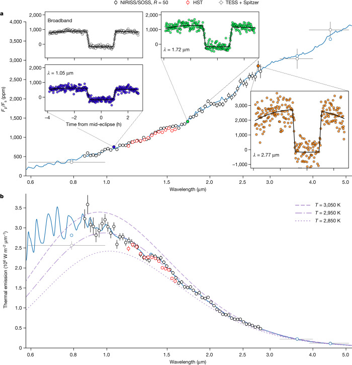
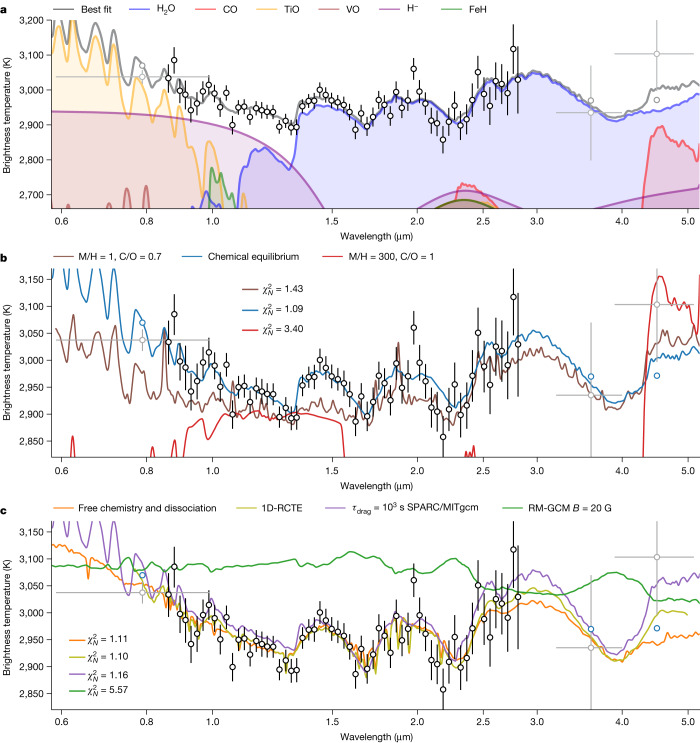
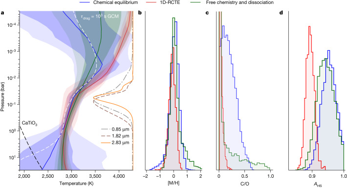
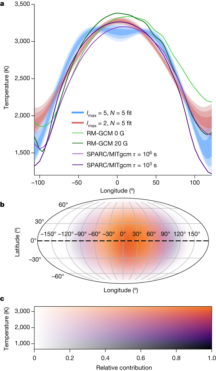
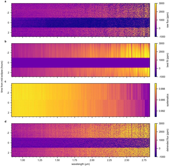
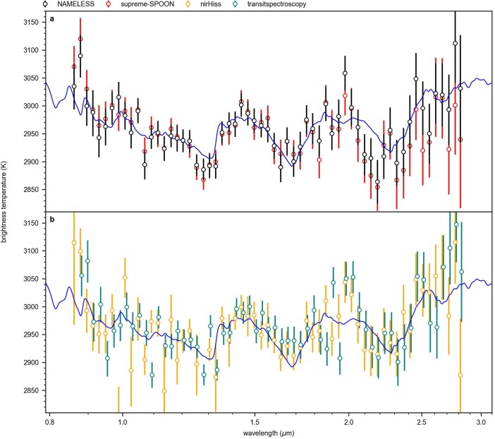
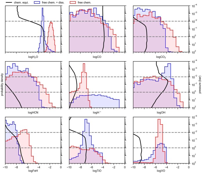
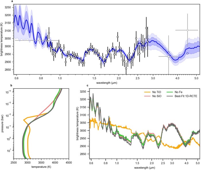
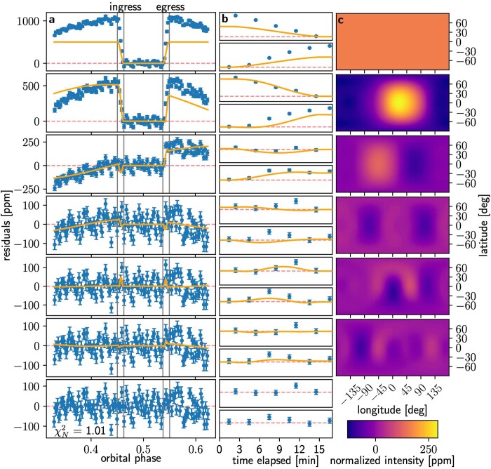
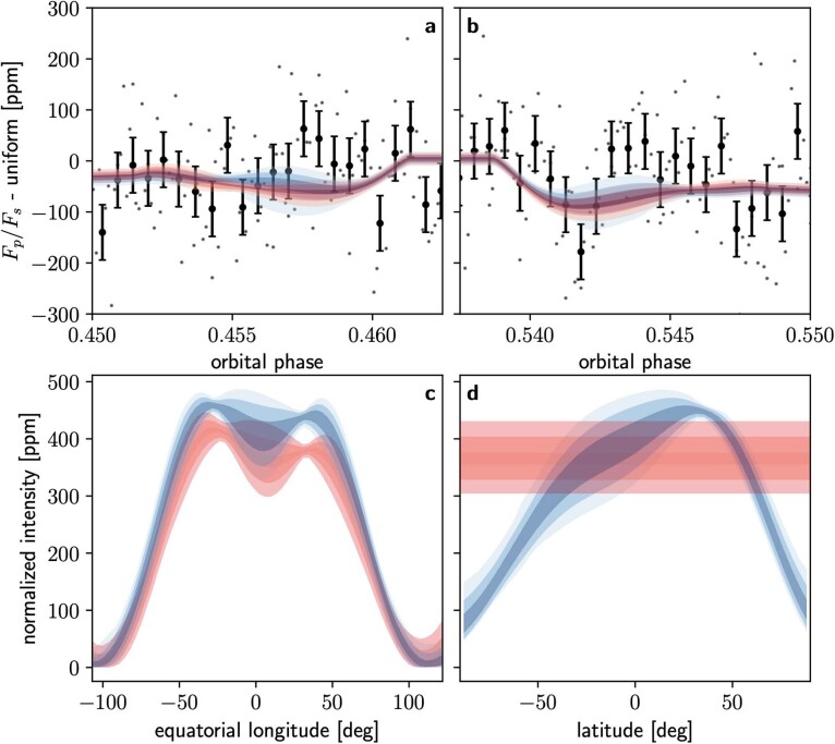
Close-in giant exoplanets with temperatures greater than 2,000 K ('ultra-hot Jupiters') have been the subject of extensive efforts to determine their atmospheric properties using thermal emission measurements from the Hubble Space Telescope (HST) and Spitzer Space Telescope^1-3. However, previous studies have yielded inconsistent results because the small sizes of the spectral features and the limited information content of the data resulted in high sensitivity to the varying assumptions made in the treatment of instrument systematics and the atmospheric retrieval analysis^3-12. Here we present a dayside thermal emission spectrum of the ultra-hot Jupiter WASP-18b obtained with the NIRISS¹³ instrument on the JWST. The data span 0.85 to 2.85 μm in wavelength at an average resolving power of 400 and exhibit minimal systematics. The spectrum shows three water emission features (at >6σ confidence) and evidence for optical opacity, possibly attributable to H^-, TiO and VO (combined significance of 3.8σ). Models that fit the data require a thermal inversion, molecular dissociation as predicted by chemical equilibrium, a solar heavy-element abundance ('metallicity', [Formula: see text] times solar) and a carbon-to-oxygen (C/O) ratio less than unity. The data also yield a dayside brightness temperature map, which shows a peak in temperature near the substellar point that decreases steeply and symmetrically with longitude towards the terminators.

Fig. 1. Dayside thermal emission spectrum of WASP-18b.

a, Observed dayside planet-to-star flux ratio spectrum (black points) and their 1σ error bars, binned at a fixed resolving power of R = 50 for visual clarity. Past HST (red points), TESS (see Methods) and Spitzer (grey points) are shown for comparison. We show the best-fit model (blue line) from the SCARLET chemical-equilibrium retrieval, extrapolated to the TESS and Spitzer wavelengths considering the same atmospheric parameters. We find that the measured spectrum is in good agreement with the past HST observations. The throughput-integrated model is shown for the TESS and Spitzer points (blue points). The white (broadband) light curve (white points) and three example spectrophotometric light curves (blue, green and orange points at 1.05, 1.72 and 2.77 μm, respectively), along with their best-fitting models (black line), are shown to scale. The phase variation of the measured planetary flux around the secondary eclipse is clearly visible. b, Planetary thermal emission spectrum of WASP-18b, as computed from the F_p/F_s spectrum and the PHOENIX stellar spectrum. The shortest wavelengths of the NIRISS/SOSS first order reach the maximum of the planetary spectral energy distribution, thereby enclosing 65% of the total thermal energy emitted by the planet. Blackbody spectra for temperatures T = 2,850 K (dotted line), 2,950 K (dash-dotted line) and 3,050 K (dashed line) are shown in purple, with the best-fitting blackbody spectrum to the NIRISS data being T = 2,950 ± 3 K. Source data

Fig. 2. Brightness temperature spectrum of WASP-18b.

a, Brightness temperature of WASP-18b as a function of wavelength, with models extrapolated to the TESS and Spitzer points considering the same atmospheric parameters. All data are plotted with their 1σ error bars. The H₂O emission features at 1.4, 1.9 and 2.5 μm are clearly visible. The increase in brightness temperature observed in the water features is indicative of a thermal inversion. We also observe a downward slope in the spectrum from 0.8 to 1.3 μm as the opacities of H⁻, TiO and VO decrease. We find that the precision of the observations at 2.4 μm is not sufficient to detect the small expected contribution from CO. b, Comparison of the high metallicity and C/O case (red), as well as the solar metallicity case with H⁻ opacity and H₂O dissociation (brown, best fit to the HST data shown in Fig. 1) that could both explain the past HST observations. We also show the SCARLET best-fit model to the NIRISS observations (blue). c, Median fits of the free-chemistry retrieval (orange) and of the self-consistent chemical-equilibrium grid retrieval (green). We also show the dayside spectra obtained by post-processing the SPARC/MITgcm (purple) and RM-GCM (green) for a drag timescale of τ_drag = 10³ s and a magnetic field strength of B = 20 G, respectively. We find that the SPARC/MITgcm better reproduces the observed features, as the RM-GCM is more isothermal. Source data

Fig. 3. Atmospheric constraints from the chemical-equilibrium and free-chemistry retrievals.

a, Retrieved temperature–pressure profiles with 1σ and 2σ contours for the chemical equilibrium with free temperature–pressure profile (blue), radiative–convective–thermochemical equilibrium (1D-RCTE, red) and free chemistry with thermal dissociation (green) retrievals. The retrieved temperature–pressure profiles are consistent between the retrievals and show an inversion in the pressure range that is constrained from the observations, as shown by the contribution functions at 0.85 (dot-dashed grey line), 1.82 (dashed brown line) and 2.83 μm (orange line). The temperature–pressure profile of WASP-18b is above the CaTiO3 condensation curve (dashed black line) at almost all pressures, which motivates the presence of a temperature inversion caused by TiO, as Ti is available in gas form. The dayside average temperature–pressure profile of the τ_drag = 10³ s SPARC/MITgcm (dashed white line) is computed from the viewing angle average of T(P)⁴ and shown for comparison. b–d, We also show the posterior probability distributions of the atmospheric metallicity [M/H] (b), C/O ratio (c) and area fraction A_HS (d). The area fraction A_HS is a scaling factor applied to the thermal emission spectrum to compensate for the possible presence of a concentrated hotspot contributing to most of the observed emission. All methods retrieve metallicities consistent with solar at 1σ. The retrieved C/O 3σ upper limits are of 0.6 and 0.2 for the chemical equilibrium with free temperature–pressure profile and the 1D-RCTE retrievals, respectively. Finally, we find that the area fraction A_HS is consistent with 1 when allowing the temperature–pressure profile to vary freely, indicating the lack of a concentrated hotspot on the dayside contributing to most of the observed emission. Source data

Fig. 4. Retrieved temperature map of WASP-18b.

a, Latitudinally averaged brightness temperatures (see Methods) of the planet along the equator. The blue and red shaded areas show solutions for l_max = 5, N = 5 and l_max = 2, N = 5 (see Methods), respectively. The effective broadband wavelength of the map, weighted by the observed flux (F_p + F_s) and instrument response, is λ = 1.27 μm. Statistically, the blue model is marginally preferred. Dark, medium and light shading denote the 1σ, 2σ and 3σ confidence regions, respectively, showing the range of model possibilities. Overplotted are several predictions from GCMs with magnetic field (green) or uniform (purple) drag timescales (see Methods). The plot only shows longitudes emitting at least 10% of the substellar flux. b, The temperature map of WASP-18b for the l_max = 5, N = 5 solution. Along the equator at −90°, 0° and 90° longitude, the temperatures are 1,744 K, 3,121 K and 2,009 K, respectively. c, The colour bar for the map shown in b. Colour represents the brightness temperature and saturation represents the relative contribution to the light curve based on its visibility. Source data

Extended Data Fig. 1. Spectrophotometric secondary-eclipse light curves of WASP-18b.

a, Raw light curves for all 408 spectrophotometric bins. b, Best-fit planetary flux measured from the light-curve fits. c, Systematics subtracted from a, consisting of a linear trend and the detrending against the tilt event and the trace morphology changes. The jump around 0.7 h before mid-eclipse comes from the fit of the flux offset caused by the tilt event. d, Raw light curves after subtraction of the best-fit systematics model. Some of the detrended light curves show sudden flux variations between wavelength bins outside of eclipse caused by correlations between the astrophysical and systematics models. Those correlations are, however, considered when computing the spectrum, as the F_p/F_s values are marginalized over the range of systematics model that fit the light curves.

Extended Data Fig. 2. Morphological changes of the spectral trace on the NIRISS detector as identified through PCA on the time series of the detector images.

a, First principal component with its eigenvalues (left) and its corresponding eigenimage (right). The tilt event occurring near the 1,336th integration can clearly be identified as the largest source of variance to the detector images. It results in a subtle change to the trace profile in the cross-dispersion direction, predominantly visible near its lower edge of the trace. b, Second principal component with its eigenvalues (left) and its corresponding eigenimage (right). The second principal component represents subtle changes in the y position of the trace throughout the time series, with the two edges of the trace trading flux. c, Third principal component with its eigenvalues (left) and its corresponding eigenimage (right). The third component represents changes in the FWHM of the trace and shows a clear beat pattern in time. The eigenimage for this component shows a trade of flux between the centre and the edges of the trace throughout the time series. Source data

Extended Data Fig. 3. Spectra from the four individual reductions.

Comparison of the brightness temperature spectra obtained by fitting with ExoTEP the four separate reductions and binned at a resolving power of R = 50. All data are plotted with their 1σ error bars. We overplot the best-fit SCARLET model (blue line) to the reductions for further comparison. All reductions are consistent within less than one standard deviation on average when compared at full resolution (408 bins). Source data

Extended Data Fig. 4. Light-curve residuals binned in time.

a, Absolute root mean square (RMS) of the residuals as a function of bin size (black line) for the white-light curve. The RMS values are plotted against the Poisson noise limit (red line), which decreases as the square root of the number of integrations contained in a single bin. We also show the theoretical 1σ error envelope of the Poisson noise. The residuals bin down to about 5 ppm for bins of 1 h and show no evidence of a noise floor, similar to what was observed from commissioning data. The broadband residuals do not perfectly follow the Poisson noise, which is indicative of remaining time correlations. b, Normalized RMS of the 408 spectrophotometric light curves considered in the analysis. We observe that the residuals follow the Poisson noise limit from bin sizes of a single integration up to bins of approximately 1 h, indicating that there are no time correlations in the residuals. We observe a slight decrease of the normalized RMS below the Poisson noise at larger bin sizes, similar to what was observed in the NIRCam and NIRSpec/G395H observations of WASP-39b (refs. ^,).

Extended Data Fig. 5. Abundance constraints from the free-chemistry retrievals.

Probability posteriors of the deep abundance of various species considered for the free chemistry and temperature with (blue, HyDRA) and without (red, POSEIDON) thermal dissociation. We also show the median retrieved VMR profiles from the chemical equilibrium with free temperature–pressure profile retrieval (black line, SCARLET). The pressure range investigated by the observations (about 0.01–1 bar; see Fig. 3) is indicated by the dashed grey lines. The only species independently detected is H₂O, which is found to be consistent with the retrieved chemical-equilibrium abundance when considering the effect of thermal dissociation. All other species considered are found to be unconstrained, although consistent with chemical-equilibrium predictions. The photosphere as predicted by our radiative–convective model is around 50 millibar, but the retrievals infer the deep molecular abundances. Source data

Extended Data Fig. 6. WASP-18b’s brightness temperature spectrum fit and source of the thermal inversion.

a, The dark blue line indicates the chemical-equilibrium median fit to the NIRISS data with its 1σ error bars (black points), with shaded blue regions showing the 1σ and 2σ credible intervals in the retrieved spectrum (medium and light blue, respectively). The spectra are extrapolated to the TESS (visible wavelengths) and the Spitzer/IRAC measurements (3.6 and 4.5 μm) observations (grey points) considering the same atmospheric parameters. b, Best-fit radiative–convective model temperature–pressure profile together with radiative–convective solutions in which specific species known to create a thermal inversion are removed from the atmosphere. Absorption by atomic iron contributes to the thermal inversion at pressures lower than 1.0 millibar, whereas TiO is responsible for the thermal inversion seen between 0.1 and 0.01 bar. SiO contributes at pressures lower than 0.1 bar. c, Best-fit radiative–convective brightness temperature spectrum (excluding area fraction) and resulting spectra when removing specific species. As shown by the change from emission to absorption features in the spectra when TiO is removed, the TiO-induced thermal inversion is that examined by our observations.

Extended Data Fig. 7. Light-curve predictions from GCMs.

a, GCM light curves compared against the data and the best-fitting eclipse-mapping model. b, Data and the GCM light curves with the eclipse-mapping model subtracted. The GCMs with strong atmospheric drag (RM-GCM B = 20 G and SPARC/MITgcm τ_drag = 10³ s) match the data better than their counterparts that have little to no drag. Source data

Extended Data Fig. 8. Components of the eclipse-mapping fit.

a, This column shows the light-curve components of the eclipse-mapping fit for l_max = 5, N = 5, overplotted on the data, which have been binned by a factor of 20 for clarity. From top to bottom, each light-curve component is subtracted from the data to illustrate the features that are fit by each component, such that the top row is the full white-light curve and the bottom row is the model residuals. The white-light curve points are plotted with their 1σ error bars. Note that all components are fit simultaneously. b, The same as column a, zoomed in to the ingress and egress of the eclipse to highlight the fine features fit by each component. c, The eigenmaps associated with the corresponding components in columns a and b that, when integrated, generate those light curves. Each map has been scaled by its best-fitting weight, such that a sum of this column would produce the best-fitting map.

Extended Data Fig. 9. Latitudinal structure in the eclipse map.

a, Ingress of the eclipse, with two models overplotted and a 1,096 ppm (white-light planet flux at mid-eclipse) uniform planet model subtracted to highlight deviations. The data (small dots) have been binned by a factor of five (dots with 1σ error bars) for clarity. The blue model is the eclipse map for l_max = 5, N = 5 presented in the text. The red model uses a constant-with-latitude Fourier series as the basis set, rather than spherical harmonics, to investigate constraints on latitudinal aspects of the map. Shaded regions denote 1σ, 2σ and 3σ quantiles. b, Same as a but for the eclipse egress. c, Planetary flux along the equator for the same two models. Note that, regardless of basis functions, we retrieve the same longitudinal structure, giving us confidence in the longitudinal brightness distribution. d, Same as c but along the substellar meridian. Both models fit the data well but find different latitudinal structure, indicating that we are unable to constrain latitudinal variation.

References

1. Baxter C, et al. A transition between the hot and the ultra-hot Jupiter atmospheres. Astron. Astrophys. 2020;639:A36. doi: 10.1051/0004-6361/201937394. - DOI
1. Mansfield M, et al. A unique hot Jupiter spectral sequence with evidence for compositional diversity. Nat. Astron. 2021;5:1224–1232. doi: 10.1038/s41550-021-01455-4. - DOI
1. Changeat Q, et al. Five key exoplanet questions answered via the analysis of 25 hot-Jupiter atmospheres in eclipse. Astrophys. J. Suppl. Ser. 2022;260:3. doi: 10.3847/1538-4365/ac5cc2. - DOI
1. Sheppard KB, et al. Evidence for a dayside thermal inversion and high metallicity for the hot Jupiter WASP-18b. Astrophys. J. Lett. 2017;850:L32. doi: 10.3847/2041-8213/aa9ae9. - DOI
1. Evans TM, et al. An ultrahot gas-giant exoplanet with a stratosphere. Nature. 2017;548:58–61. doi: 10.1038/nature23266. - DOI - PubMed