A plausible identifiable model of the canonical NF-κB signaling pathway

Abstract

An overwhelming majority of mathematical models of regulatory pathways, including the intensively studied NF-κB pathway, remains non-identifiable, meaning that their parameters may not be determined by existing data. The existing NF-κB models that are capable of reproducing experimental data contain non-identifiable parameters, whereas simplified models with a smaller number of parameters exhibit dynamics that differs from that observed in experiments. Here, we reduced an existing model of the canonical NF-κB pathway by decreasing the number of equations from 15 to 6. The reduced model retains two negative feedback loops mediated by IκBα and A20, and in response to both tonic and pulsatile TNF stimulation exhibits dynamics that closely follow that of the original model. We carried out the sensitivity-based linear analysis and Monte Carlo-based analysis to demonstrate that the resulting model is both structurally and practically identifiable given measurements of 5 model variables from a simple TNF stimulation protocol. The reduced model is capable of reproducing different types of responses that are characteristic to regulatory motifs controlled by negative feedback loops: nearly-perfect adaptation as well as damped and sustained oscillations. It can serve as a building block of more comprehensive models of the immune response and cancer, where NF-κB plays a decisive role. Our approach, although may not be automatically generalized, suggests that models of other regulatory pathways can be transformed to identifiable, while retaining their dynamical features.

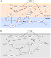
Fig 1. NF-κB pathway diagrams.

(A) Diagram of the 15-variable original model. The short lasting cytoplasmic complexes (IKK|IκBα) and (IKK|NF-κB|IκBα) are not depicted for the sake of simplicity. The bold arrows represent the fast dynamics. (B) Diagram of the reduced 6-variable model. NF-κB* denoting cytoplasmic (NF-κB|IκBα) complexes is not associated with the separate equation, since the amount of total NF-κB remains constant: NFκB_n + NFκB* = 1.

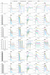
Fig 2. Dynamics of the original, reduced and reduced fitted models in the combination experiment defined in S1 Table.

Red dots indicate time points from which the nuclear NF-κB and total IκBα protein in silico measurements are used for fitting the reduced model to the original one. The time points for the remaining variables are given in S1 Table.

Fig 3. Simulations of the original model for five different sets of parameters and the corresponding reduced model with refitted parameter values (see S3 and S4 Tables).

Simulations are performed for the combination experiment defined in S1 Table. For each parameter set the corresponding ${\text{AMD}}_{WT}^{*}$ is computed based on trajectories of the 5 main model variables. Each color corresponds to a different parameter set; for each parameter set, a continuous line shows the original model trajectory, while a thinner dashed line shows the corresponding trajectory of the reduced model with refitted parameters.

Fig 4. Structural identifiability analysis of the reduced and original models.

Singular values of the sensitivity matrices S for the original and reduced models. Graphs show all 23 scaled singular values obtained (for the combination experiment) for the original model vs. 13 singular values obtained for the reduced model. Singular values, arranged in descending order, in the original model reveal a clear gap, indicating that the corresponding sensitivity matrix is rank deficient and hence the original model is structurally non-identifiable.

Fig 5. Linear identifiability analysis of the reduced model.

(A) Comparison of the three smallest scaled singular values computed for different protocols. (B) Smallest scaled norms of sensitivity vectors ||S_j||. (C) Three smallest scaled norms of perpendicular components $\left|\right|S_j^{\perp |}\left|\right|$. (D) Three largest scaled ratios of the parameter estimation error to experimental error R_j = ln(σ_linear,j)/ln(σ_data). The combination experiment includes the continuous and 5 pulsatile protocols. Scaling with $\sqrt{dim}$ allows to compare the protocols having a different dimension of sensitivity vectors.

Fig 6. Identifiability analysis of the reduced model—comparison of the protocols: Continuous, combination experiment and on–off.

(A) Scaled singular values. (B) Scaled norms of sensitivity vectors ||S_j||. (C) Scaled norms of perpendicular components $\left|\right|S_j^{\perp }\left|\right|$. (D) Scaled ratios of parameter estimation error to experimental error ln(σ_linear,j)/ln(σ_data). Scaling with $\sqrt{dim}$ allows for a comparison of the three protocols having a different dimension of sensitivity vectors.

Fig 7. Practical identifiability of the reduced model based on Monte Carlo simulations.

(A) A comparison of 75% confidence ellipses (shown in black) computed for σ_data = 1.3 in the linear sensitivity matrix based analysis with results from 50 Monte Carlo simulations for four values of σ_data (1.0, 1.1, 1.2, 1.3). Shown are projections on 15 planes spanned by 6 parameters with the largest geometric standard deviations σ_carlo,j (for σ_data = 1.3). (B) The geometric standard deviation of parameter estimation error σ_carlo,j obtained in Monte Carlo simulation for four values of geometric standard deviations of measurements, σ_data (1.0, 1.1, 1.2, 1.3), is compared with the geometric standard deviation of parameter estimation σ_linear,j obtained from the linear analysis for σ_data = 1.3.

Fig 8. Three types of the oscillatory responses of the reduced model to tonic TFN stimulation: Left subpanels show nuclear NFκB_n(t) in response to tonic TNF stimulation started at t = 1 hour, whereas the right subpanels show trajectories projected on the (NFκB_n, IκBα) plane.

(A) Damped oscillations observed for the nominal (fitted to the original model) parameters values (see Table 1), in particular a₂ = 0.0762, c_5a = 0.000058, i_1a = 0.000595 (modified in panels B and C). The black dot on right subpanel shows the ‘T_R = 1’ stable steady state. (B) Limit cycle oscillations of nuclear NFκB_n(t) observed in simulations performed for a₂ = 0.02, c_5a = 0.00001, i_1a = 0.0001 and other parameters unchanged. The orange dot on the right subpanel shows the ‘T_R = 1’ unstable steady state surrounded by a stable limit cycle (black line). A numerically computed orbit (shown in red) approaches the stable limit cycle. (C) Periodic relaxation-like oscillations observed in simulations performed for a₂ = 0.01, c_5a = 0.00001, i_1a = 0.0001 and other parameters unchanged. Again, the orange dot on the right subpanel shows the ‘T_R = 1’ unstable steady state surrounded by a stable limit cycle (black line).

Fig 9. Influence of A20 feedback on the reduced model responses to tonic TNF stimulation.

Left subpanels show nuclear NFκB_n(t) in response to tonic TNF stimulation started at t = 1 hour, whereas the right subpanels show trajectories projected on the (NFκB_n, IκBα) or (NFκB_n, A20) planes. (A) Numerically computed solution for k₂ = 0 (and other parameters unchanged, as in Table 1) implying absence of A20 mediated feedback (as in A20 KO cells). (B) Nearly-perfect adaptation observed in the model variant with significantly stronger negative feedbacks mediated by A20 and IκBα. Numerical simulations are performed for k₂ = 3.57 and i_1a = 0.01 (changed from the nominal values k₂ = 0.0357 and i_1a = 0.00595) and other parameters unchanged.

References

1. Wieland F-G, Hauber AL, Rosenblatt M, Tönsing C, Timmer J. On structural and practical identifiability. Curr Opin Syst Biol. 2021; 25:60–9. doi: 10.1016/j.coisb.2021.03.005 - DOI
1. Anguelova M, Karlsson J, Jirstrand M. Minimal output sets for identifiability. Math Biosci. 2012; 239(1):139–153. doi: 10.1016/j.mbs.2012.04.005 - DOI - PubMed
1. Joubert D, Stigter JD, Molenaar J. Determining minimal output sets that ensure structural identifiability. PLoS ONE. 2018; 13(11):e0207334 (2018). doi: 10.1371/journal.pone.0207334 - DOI - PMC - PubMed
1. Nienałtowski K, Włodarczyk M, Lipniacki T, Komorowski M. Clustering reveals limits of parameter identifiability in multi-parameter models of biochemical dynamics. BMC Syst Biol. 2015; 9(1):65. doi: 10.1186/s12918-015-0205-8 - DOI - PMC - PubMed
1. Lipniacki T, Paszek P, Brasier AR, Luxon B, Kimmel M. Mathematical model of NF-κB regulatory module. J Theor Biol. 2004; 228(2):195–215. doi: 10.1016/j.jtbi.2004.01.001 - DOI - PubMed
Publication types