Deep learning-based Lorentzian fitting of water saturation shift referencing spectra in MRI

Abstract

Purpose: Water saturation shift referencing (WASSR) Z-spectra are used commonly for field referencing in chemical exchange saturation transfer (CEST) MRI. However, their analysis using least-squares (LS) Lorentzian fitting is time-consuming and prone to errors because of the unavoidable noise in vivo. A deep learning-based single Lorentzian Fitting Network (sLoFNet) is proposed to overcome these shortcomings.

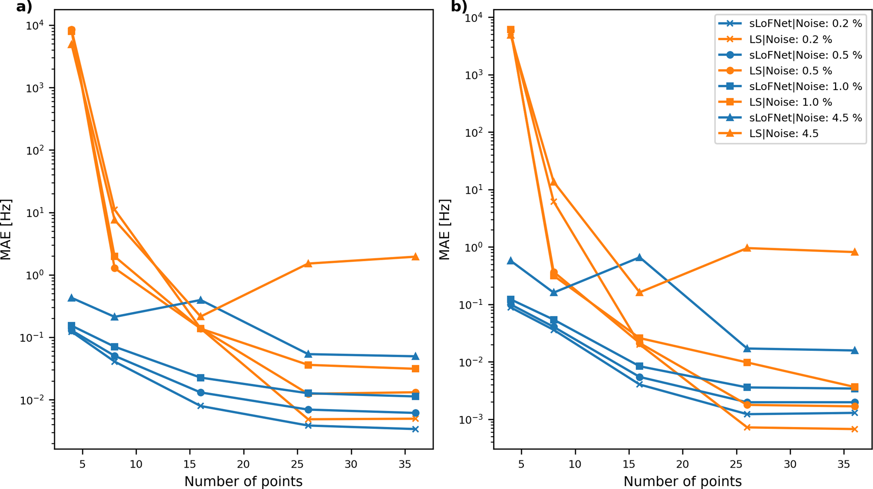
Methods: A neural network architecture was constructed and its hyperparameters optimized. Training was conducted on a simulated and in vivo-paired data sets of discrete signal values and their corresponding Lorentzian shape parameters. The sLoFNet performance was compared with LS on several WASSR data sets (both simulated and in vivo 3T brain scans). Prediction errors, robustness against noise, effects of sampling density, and time consumption were compared.

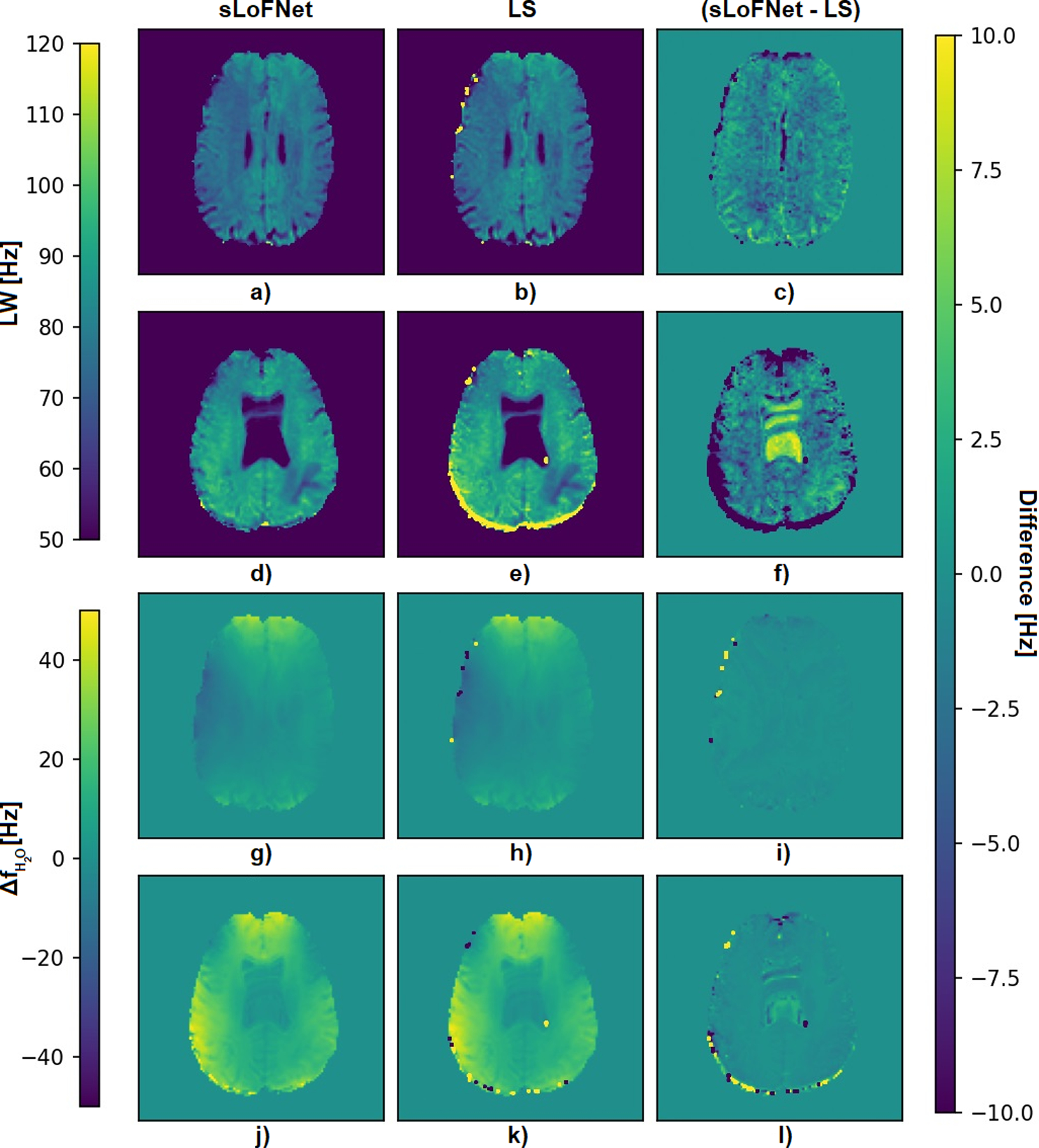
Results: LS and sLoFNet performed comparably in terms of RMS error and mean absolute error on all in vivo data with no statistically significant difference. Although the LS method fitted well on samples with low noise, its error increased rapidly when increasing sample noise up to 4.5%, whereas the error of sLoFNet increased only marginally. With the reduction of Z-spectral sampling density, prediction errors increased for both methods, but the increase occurred earlier (at 25 vs. 15 frequency points) and was more pronounced for LS. Furthermore, sLoFNet performed, on average, 70 times faster than the LS-method.

Conclusion: Comparisons between LS and sLoFNet on simulated and in vivo WASSR MRI Z-spectra in terms of robustness against noise and decreased sample resolution, as well as time consumption, showed significant advantages for sLoFNet.

Keywords: Lorentzian fitting; WASSR; Z-spectra; deep learning; least squares.

Figure 1.

An overview of the project’s workflow.

Figure 2.

(a) The RMSE combining the errors in amplitude, linewidth, and shift of training (blue) and validation (orange) data for the optimized network (sLoFNet_HP) as a function of the number of completed training epochs. (b) Performance in terms of RMSE of sLoFNet_HP (at 5 000 000 training samples), sLoFNet₃ (at 500 000 training samples), sLoFNet₂ (at 50 000 training samples) and sLoFNet₁ (at 5000 training samples) on the training (blue), validation (orange) and test (green) datasets. The upper horizontal axis shows the increasing training time with increased number of training samples. Note the logarithmic scale on the x-axis in (b).

Figure 3.

The MAE of the sLoFNET_HP predictions (blue), sLoFNET_Invivo predictions (green), and LS estimations (orange) as a function of noise level of the datasets. (a) the combined error, (b) the error in amplitude, (c) the error in LW and (d) the error in shift.

Figure 4.

The Lorentzian fits on representative in vivo voxel examples from (a) CSF (LW [Hz]: sLoFNet_HP, LS, sLoFNet_Invivo = 84.1, 84.7, 85.2 and ${\Delta \text{f}}_{{\text{H}}_2\text{O}}$ [Hz]: sLoFNet_HP, LS, sLoFNet_Invivo = 4.35, 4.48, 4.39). (b) WM (LW [Hz]: sLoFNet_HP, LS, sLoFNet_Invivo = 83.8, 84.5, 84.4 and ${\Delta \text{f}}_{{\text{H}}_2\text{O}}$ [Hz]: sLoFNet_HP, LS, sLoFNet_Invivo = −1.66, −1.66, −1.75). (c) GM (LW [Hz]: sLoFNet_HP, LS, sLoFNet_Invivo = 82.0, 82.4, 86.7 and ${\Delta \text{f}}_{{\text{H}}_2\text{O}}$ [Hz]: sLoFNet_HP, LS, sLoFNet_Invivo = 12.9, 13.0, 12.6) Voxels are indicated in the respective FLAIR images. The fits of sLoFNet_HP (blue), LS (orange) and sLoFNet_Invivo (green) overlap within the line thickness. (d)-(f) The corresponding signal intensity differences between the sLoFNet_HP, LS, and sLoFNet_Invivo fits. For visual separation purposes, we display sLoFNet_HP – LS and LS - sLoFNet_Invivo.

Figure 5.

(a)-(c) Examples of the good agreement between the sLoFNet_HP fitted line (blue), the LS fitted line (orange) and sLoFNet_Invivo (green) for voxels from T_GBM, T_RMS and, T_MM (marked in the FLAIR images). (d)-(f) Examples of poor fits on voxel samples from T_GBM, T_RMS and, T_MM.

Figure 6.

Examples of parameter maps. Healthy volunteer: (a), (b) and (c) show LW and (g), (h) and (i) show shift. Rhabdomyosarcoma metastasis patient: (d), (e) and (f) show LW and (j), (k), (l) show shift. The first column is produced by the sLoFNet_HP, the second by the LS-method and the third is the difference between the two methods (sLoFNet_HP-LS).

Figure 7.

The prediction errors (MAE in Hz) for (a) LW and (b) $\Delta f_{H_{2}O}$ as a function of the number of points in the samples for sLoFNet_HP (blue) and LS (orange). The different curves indicate different noise levels for the samples used for prediction (✖ - 0.2%, ● – 0.5%, ■ – 1.0% and ▲- 4.5%)

Figure 8.

The prediction errors (MAE in Hz) as a function of WSW-to-LW ratio for (a) the predicted LW and (b) the predicted shift. The different curves show samples with a different number of points (✖ 4, ● 8, ■ 16, ▲26 and ▼36) using sLoFNet_HP (blue) and LS (orange).